Range Analysis Domain for BigInt

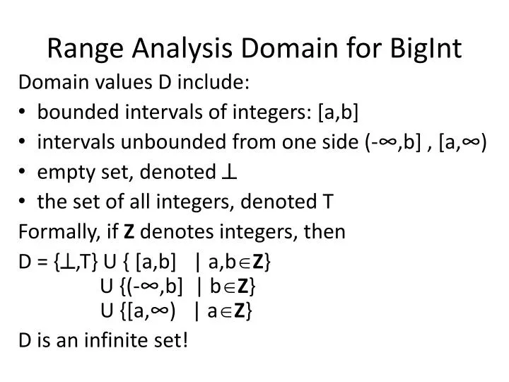
Range Analysis Domain for BigInt Domain values D include: • bounded intervals of integers:[a,b] • intervals unbounded from one side (-∞,b] , [a,∞) • empty set, denoted  • the set of all integers, denoted T Formally, if Z denotes integers, then D = {,T} U { [a,b] | a,bZ} U {(-∞,b] | bZ} U {[a,∞) | aZ} D is an infinite set!

Sequences in Analysis are Monotonically Growing Transfer functions (describe how statements affect elements of D) should be monotonic: if we start with a representation of a larger set of states, the representation of the resulting set of states should also be larger x = x + 2 d1 ≤ d2 implies [[x=x+2]](d1) ≤ [[x=x+2]](d2) We start from everywhere except entry So in first step, the values can only grow ≤ d2 implies [[x=x+2]]() ≤ [[x=x+2]](d2) Values computed in second step are also bigger If xn = Fn() then x0 =  ≤ x1 xn ≤ xn+1 / F F(xn)≤ F(xn+1)i.e. xn+1≤ xn+2 x: [a,b] x: [a+2,b+2]

How Long Does Analysis Take? • We explore this question by comparing • range analysis: maintain intervals • constant propagation: maintains indication whether the value is constant

Iterating Range Analysis Find the number of updates range analysis needs to stabilize in the following code x = 1 while (x < n) { x = x + 2 } n = 1000

Iterating Range Analysis Now, if we assume that any number can be entered from the user, what is now the number of steps? x = 1 while (x < n) { x = x + 2 } n = readInput() //anything, so n becomes T For unknown program inputs and unbounded domains, such analysis need not terminate! One solution: “smaller” domain

Range Analysis with Finite Set of Endpoints Pick a set W of “interesting” interval end-points Example: W = {-128, 0, 127} D = {,T} U { [a,b] | a,bW, a ≤ b} U {(-∞,b] | b W} U {[a,∞) | a W} D is a finite set! How many elements does it have?

Domain Lattice Diagram for this W: 14 elements T ∞ ∞ ∞ ∞ ∞ ∞ ∞ ∞

Re-Run Analysis with Finite Endpoint Set What is the number of updates? x = 1n = 1000 while (x < n) { x = x + 2 } x = 1n = readInt() while (x < n) { x = x + 2 }

Constant Propagation Domain Domain values D are: • intervals [a,a], denoted simply ‘a’ • empty set, denoted  and set of all integers T Formally, if Z denotes integers, then D = {,T} U { a | aZ} D is an infinite set T 0 2 • … 1 -2 -1 • … 

Constant Propagation Transfer Functions table for +: x = y + z For each variable (x,y,z) and each CFG node (program point)we store:  ,a constant, or T abstract class Element case class Top extends Element case class Bot extends Element case class Const(v:Int) extends Element var facts : Map[Nodes,Map[VarNames,Element]] what executes during analysis of x=y+z : oldY = facts(v1)("y") oldZ = facts(v1)("z") newX = tableForPlus(oldY, oldZ) facts(v2) = facts(v2) join facts(v1).updated("x", newX) deftableForPlus(y:Element, z:Element) = (x,y) match {case (Const(cy),Const(cz)) => Const(cy+cz)case (Bot,_) => Botcase (_,Bot) => Botcase (Top,Const(cz)) => Topcase (Const(cy),Top) => Top}

Run Constant Propagation What is the number of updates? x = 1 while (x < n) { x = x + 2 } x = 1n = readInt() while (x < n) { x = x + 2 } n = 1000

Observe • Range analysis with W = {-128, 0, 127} has a finite domain • Constant propagation has infinite domain (for every integer constant, one element) • Yet, constant propagation finishes sooner! • it is not about the size of the domain • it is about the height

Height of Lattice: Length of Max. Chain height=5 size=14 T ∞ ∞ ∞ ∞ ∞ ∞ ∞ ∞ T height=2 size =∞ 0 2 • … 1 -2 -1 • … 

Chain of Length n • A set of elements x0,x1 ,..., xnin D that are linearly ordered, that is x0<x1< ...< xn • A lattice can have many chains. Its height is the maximum n for all the chains • If there is no upper bound on lengths of chains, we say lattice has infinite height • Any monotonic sequence of distinct elements has length at most equal to lattice height • including sequence occuring during analysis! • such sequences are always monotonic

In constant propagation, each value can change only twice T • consider value for x before assignment • Initially:  • changes 1st time to: 1 • change 2nd time to: T • total changes: two (height) x = 1n = 1000 while (x < n) { x = x + 2 } height=2 size =∞ 0 2 • … 1 -2 -1 • … var facts : Map[Nodes,Map[VarNames,Element]]  • Total number of changes bounded by: height∙|Nodes| ∙|Vars|

Exercise B32– the set of all 32-bit integers What is the upper bound for number of changes in the entire analysis for: • 3 variables, • 7 program points for these two analyses: • constant propagation for constants from B32 • The following domain D: D = {} U { [a,b] | a,bB32 ,a ≤ b}

Height of B32 D = {} U { [a,b] | a,b B32 ,a ≤ b} One possible chain of maximal length:  … [MinInt,MaxInt]

Initialization Analysis first initialization uninitialized initialized

What does javac say to this: class Test { static void test(int p) { intn; p = p - 1; if (p > 0) { n = 100; } while (n != 0) { System.out.println(n); n = n - p; } } } Test.java:8: variable n might not have been initialized while (n > 0) { ^ 1 error

Program that compiles in java We would like variables to be initialized on all execution paths. Otherwise, the program execution could be undesirable affected by the value that was in the variable initially. We can enforce such check using initialization analysis. class Test { static void test(int p) { intn; p = p - 1; if (p > 0) { n = 100; } else { n = -100; } while (n != 0) { System.out.println(n); n = n - p; } } }

What does javac say to this? static void test(int p) { int n; p = p - 1; if (p > 0) { n = 100; } System.out.println(“Hello!”); if (p > 0) { while(n != 0) { System.out.println(n); n = n - p; } } }

Initialization Analysis class Test { static void test(int p) { intn; p = p - 1; if (p > 0) { n = 100; } else { n = -100; } while (n != 0) { System.out.println(n); n = n - p; } } } T indicates presence of flow from states where variable was not initialized: • If variable is possibly uninitialized, we use T • Otherwise (initialized, or unreachable):  If var occurs anywhere but left-hand sideof assignment and has value T, report error

Sketch of Initialization Analysis • Domain: for each variable, for each program point: D = {,T} • At program entry, local variables: T ; parameters:  • At other program points: each variable:  • An assignment x = e sets variable x to  • lub (join, ) of any value with T gives T • uninitialized values are contagious along paths •  value for x means there is definitely no possibility for accessing uninitialized value of x

Run initialization analysis Ex.1 int n; p = p - 1; if (p > 0) { n = 100; } while (n != 0) { n = n - p; }

Run initialization analysis Ex.2 int n; p = p - 1; if (p > 0) { n = 100; } if (p > 0) { n = n - p; }

Liveness Analysis Variable is dead if its current value will not be used in the future.If there are no uses before it is reassigned or the execution ends, then the variable is surely dead at a given point. first initialization last use live live dead dead dead

Example: What is Written and What Read x = y + x if (x > y) Purpose: Register allocation: find good way to decide which variable should go to which register at what point in time.

How Transfer Functions Look

Initialization: Forward Analysis while (there was change)pick edge (v1,statmt,v2) from CFG such that facts(v1) has changed facts(v2)=facts(v2) jointransferFun(statmt, facts(v1))} Liveness: Backward Analysis while (there was change)pick edge (v1,statmt,v2) from CFG such that facts(v2) has changed facts(v1)=facts(v1) jointransferFun(statmt, facts(v2))}

Example x = m[0] y = m[1] xy = x * y z = m[2] yz = y*z xz = x*z res1 = xy + yz m[3] = res1 + xz

Data Representation Overview

Original and Target Program have Different Views of Program State • Original program: • local variables given by names (any number of them) • each procedure execution has fresh space for its variables (even if it is recursive) • fields given by names • Java Virtual Machine • local variables given by slots (0,1,2,…), any number • intermediate values stored in operand stack • each procedure call gets fresh slots and stack • fields given by names and object references • Machine code: program state is a large array of bytes and a finite number of registers

Compilation Performs Automated Data Refinement Data Refinement FunctionR x  0y  5z  8 1 02  53  8 c s iload2iconst 7 iload 3 imul iadd istore 1 P: x = y + 7 * z x  61y  5z  8 [[x = y + 7 * z]] = s’ R maps s to cand s’ to c’ 1 612  53  8 If interpreting program Pleads from s to s’then running the compiled code [[P]]leads from R(s) to R(s’) c'

Inductive Argument for Correctness 0 01  52  8 x  0y  5z  8 R c1 s1 [[x = y + 7 * z]] x = y + 7 * z 0 611  52  8 x  61y  5z  8 R c2 s2 iload 3; iconst 1; iadd; istore 2 y = z + 1 0 611  92  8 x  61y  9z  8 R c3 s3 (R may need to be a relation, not just function)

A Simple Theorem P : S  S is a program meaning function Pc : C  C is meaning function for the compiled program R : S  Cis data representation functionLet sn+1 = P(sn), n = 0,1,… be interpreted executionLet cn+1= P(cn), n = 0,1,… be compiled execution Theorem: If • c0 = R(s0) • for all s, Pc(R(s)) = R(P(s)) then cn = R(cn) for all n. Proof: immediate, by induction. R is often called simulation relation.

Example of a Simple R • Let the receiver, the parameters, and local variables, in their order of declaration, be x1, x2 … xn • Then R maps program state with only integers like this: x1 v1x2  v2x3  v3 … xn vn 0  v11  v22  v3 … (n-1) vn R

R for Booleans • Let the received, the parameters, and local variables, in their order of declaration, be x1, x2 … xn • Then R maps program state like this, where x1 and x2 are integers but x3 and x4 are Booleans: x1 3x2  9x3  true x4 false 0  31  92  1 3  0 R

R that depends on Program Point x  v1res  v2 y  v3z  v4 0  v11  v2 2  v33  v4 def main(x:Int) {var res, y, z: Intif (x>0) { y = x + 1 res = y } else { z = -x - 10 res = z } return res;} R x  v1res  v2 y  v3z  v4 0  v11  v2 2  v3 R1 x  v1res  v2 y  v3z  v4 0  v11  v2 2  v4 R2 Map y,z to same slot. Consume fewer slots!

Packing Variables into Memory • If values are not used at the same time, we can store them in the same place • This technique arises in • Register allocation: store frequently used values in a bounded number of fast registers • ‘malloc’ and ‘free’ manual memory management: free releases memory to be used for later objects • Garbage collection, e.g. for JVM, and .NET as well as languages that run on top of them (e.g. Scala)

Register Machines Directly Addressable RAM (large - GB,slow, even with caches) Better for most purposes than stack machines • closer to modern CPUs (RISC architecture) • closer to control-flow graphs • simpler than stack machine Example: ARM architecture R0,R1,…,R31 A few fastregisters

Basic Instructions of Register Machines Ri  Mem[Rj] load Mem[Rj] Ristore Ri Rj * Rkcompute: for an operation * Efficient register machine code uses as few loads and stores as possible.

State Mapped to Register Machine Both dynamically allocated heap and stack expand • heap need not be contiguous; can request more memory from the OS if needed • stack grows downwards Heap is more general: • Can allocate, read/write, and deallocate, in any order • Garbage Collector does deallocationautomatically • Must be able to find free space among used one, group free blocks into larger ones (compaction),… Stack is more efficient: • allocation is simple: increment, decrement • top of stack pointer (SP) is often a register • if stack grows towards smaller addresses: • to allocate N bytes on stack (push): SP := SP - N • to deallocate N bytes on stack (pop): SP := SP + N 1 GB Stack SP free memory 10MB Heap Constants 50kb Static Globals 0 Exact picture maydepend on hardware and OS

JVM vs General Register Machine CodeNaïve Correct Translation R1  Mem[SP] SP = SP + 4 R2  Mem[SP] R2  R1 * R2 Mem[SP]  R2 JVM: Register Machine: imul

Register Allocation

How many variables? x,y,z,xy,xz,res1 Do we need 6 distinct registersif we wish to avoid load and stores? x = m[0] y = m[1] xy = x * y z = m[2] yz = y*z xz = x*z res1 = xy + yz m[3] = res1 + xz x = m[0] y = m[1] xy = x * y z = m[2] yz = y*z y = x*z // reuse y x = xy + yz// reuse x m[3] = x + y can do it with 5 only! 7 variables:x,y,z,xy,yz,xz,res1

Range Analysis Domain for BigInt