Download
1 / 35
350 likes | 498 Views
Succinct Representations of Trees. S. Srinivasa Rao IT University of Copenhagen. Outline. Succinct data structures Introduction Examples Tree representations Heap-like representation Jacobson’s representation Parenthesis representation Partitioning method Conclusions.

E N D
Succinct Representations of Trees S. Srinivasa Rao IT University of Copenhagen
Outline • Succinct data structures • Introduction • Examples • Tree representations • Heap-like representation • Jacobson’s representation • Parenthesis representation • Partitioning method • Conclusions
Succinct data structures • Goal: represent the data in close to optimal space, while supporting the operations efficiently. (optimal –– information-theoretic lower bound) • An “extension” of data compression. (Data compression: • Achieve close to optimal space • Queries need not be supported efficiently. )
Applications • Potential applications where • memory is limited: small memory devices like PDAs, mobile phones etc. • massive amounts of data: DNA sequences, geographical/astronomical data, search engines etc.
Examples • Trees, Graphs • Bit vectors, Sets • Dynamic arrays • Text indexes • suffix trees/suffix arrays etc. • Permutations, Functions • XML documents, File systems (labeled, multi-labeled trees) • BDDs • …
(1)=6 -1(1)=5 1 2 3 4 5 6 7 8 : 6 5 2 8 1 3 4 7 Example: Permutations A permutation of 1,…,n A simple representation: • n lg n bits • (i) in O(1) time • -1(i) in O(n) time Our representation: • (1+ε) n lg n bits • (i) in O(1) time • -1(i) in O(1/ε) time (`optimal’ trade-off) • k(i) in O(1/ε) time (for any positive or negative integer k) • lg (n!) + o(n) (< n lg n) bits (optimal space) • k(i) in O(lg n / lg lg n) time 2(1)=3 -2(1)=5 …
Example: Functions • A function f : {1,…,n} → {1,…,n} can be represented - using n lg n + O(n) bits - fk(i) in O(1) time - f-k(i) in O(1+|output|) time (optimal space and query times). • Can also be generalized to arbitrary functions (f : {1,…,n} → {1,…,m}).
Motivation Trees are used to represent: - Directories (Unix, all the rest) - Search trees (B-trees, binary search trees, digital trees or tries) - Graph structures (we do a tree based search) • Search indexes for text (including DNA) • Suffix trees • XML documents • …
Space for trees • The space used by the tree structure could be the dominating factor in some applications. • Eg. More than half of the space used by a standard suffix tree representation is used to store the tree structure. • Standard representations of trees support very few operations. To support other useful queries, they require a large amount of extra space.
Standard representation Binary tree: each node has two pointers to its left and right children An n-node tree takes 2n pointers or 2n lg n bits (can be easily reduced to n lg n + O(n) bits). Supports finding left child or right child of a node (in constant time). For each extra operation (eg. parent, subtree size) we have to pay, roughly, an additional n lg n bits. x x x x x x x x x
Can we improve the space bound? • There are less than 22ndistinct binary trees on n nodes. • 2n bits are enough to distinguish between any two different binary trees. • Can we represent an n node binary tree using 2n bits?
Heap-like notation for a binary tree 1 Add external nodes 1 1 Label internal nodes with a 1 and external nodes with a 0 1 0 1 1 0 1 0 0 1 0 Write the labels in level order 1 1 1 1 0 1 1 0 1 0 0 1 0 0 0 0 0 0 0 0 0 One can reconstruct the tree from this sequence An n node binary tree can be represented in 2n+1 bits. What about the operations?
Heap-like notation for a binary tree 1 left child(x) = [2x] 1 2 3 2 3 right child(x) = [2x+1] 4 5 6 7 4 5 6 parent(x) = [⌊x/2⌋] 12 8 9 10 11 13 7 8 x x: # 1’s up to x x x: position of x-th 1 14 15 16 17 1 2 3 4 5 6 7 8 1 1 1 1 0 1 1 0 1 0 0 1 0 0 0 0 0 1 2 3 4 5 6 7 8 9 10 11 12 13 14 15 16 17
Rank/Select on a bit vector Given a bit vector B rank1(i) = # 1’s up to position i in B select1(i) = position of the i-th 1 in B (similarly rank0 and select0) 1 2 3 4 5 6 7 8 9 10 11 12 13 14 15 B: 0 1 1 0 1 0 0 0 1 1 0 1 1 1 1 rank1(5)= 3 select1(4)= 9 rank0(5) = 2 select0(4)= 7 Given a bit vector of length n, by storing an additional o(n)-bit structure, we can support all four operations in constant time. An important substructure in most succinct data structures. Have been implemented.
Binary tree representation • A binary tree on n nodes can be represented using 2n+o(n) bits to support: • parent • left child • right child in constant time.
Ordered trees A rooted ordered tree (on n nodes): Navigational operations: - parent(x)= a - first child(x)= b -next sibling(x)= c Other useful operations: -degree(x)= 2 -subtree size(x)= 4 a x c b
Ordered trees • A binary tree representation taking 2n+o(n) bits that supports parent, left childand right child operations in constant time. • There is a one-to-one correspondence between binary trees (on n nodes) and rooted ordered trees (on n+1 nodes). • Gives an ordered tree representation taking 2n+o(n) bits that supports first child, next sibling (but not parent) operations in constant time. • We will now consider ordered tree representations that support more operations.
Level-order degree sequence 3 Write the degree sequence in level order 3 2 0 3 0 1 0 2 0 0 0 0 2 0 3 But, this still requires n lg n bits 0 1 0 2 0 Solution: write them in unary 1 1 1 0 1 1 0 0 1 1 1 0 0 1 0 0 1 1 0 0 0 0 0 Takes 2n-1 bits 0 0 0 A tree is uniquely determined by its degree sequence
Supporting operations Add a dummy root so that each node has a corresponding 1 1 0 1 1 1 0 1 1 0 0 1 1 1 0 0 1 0 0 1 1 0 0 0 0 0 1 2 3 4 5 6 7 8 9 10 11 12 1 node k corresponds to the k-th 1 in the bit sequence 3 4 2 parent(k) = # 0’s up to the k-th 1 children of k are stored after the k-th 0 7 9 5 6 8 supports: parent, i-th child, degree (using rank and select) 10 11 12
Level-order unary degree sequence • Space: 2n+o(n) bits • Supports • parent • i-th child (and hence first child) • next sibling • degree in constant time. Does not support subtree size operation. [Implementation: Delpratt-Rahman-Raman, WAE-06]
Another approach Write the degree sequence in depth-first order 3 3 2 0 1 0 0 3 0 2 0 0 0 2 0 3 0 1 0 2 0 In unary: 1 1 1 0 1 1 0 0 1 0 0 0 1 1 1 0 0 1 1 0 0 0 0 Takes 2n-1 bits. 0 0 0 The representation of a subtree is together. Supports subtree size along with other operations. (Apart from rank/select, we need some additional operations.)
Depth-first unary degree sequence • Space: 2n+o(n) bits • Supports • parent • i-th child (and hence first child) • next sibling • degree • subtree size in constant time.
Other useful operations 1 XML based applications: level ancestor(x,l):returns the ancestor of x at level l eg.level ancestor(11,2) = 4 3 4 2 7 9 5 6 8 Suffix tree based applications: LCA(x,y): returns the least common ancestor of x and y eg.LCA(7,12) = 4 10 11 12
Parenthesis representation Associate an open-close parenthesis-pair with each node ( ) Visit the nodes in pre-order, writing the parentheses ( ) ( ) ( ) length: 2n ( ) ( ) ( ) ( ) ( ) space: 2n bits One can reconstruct the tree from this sequence ( ) ( ) ( ) ( ( ( ) ( ( ) ) ) ( ) ( ( ) ( ( ) ( ) ) ( ) ) )
Operations 1 parent– enclosing parenthesis first child – next parenthesis (if ‘open’) 3 4 2 next sibling– open parenthesis following the matching closing parenthesis (if exists) 7 9 5 6 8 subtree size – half the number of parentheses between the pair with o(n) extra bits, all these can be supported in constant time 10 11 12 ( ( ( ) ( ( ) ) ) ( ) ( ( ) ( ( ) ( ) ) ( ) ) ) 1 2 5 6 10 3 4 7 8 11 12 9
Parenthesis representation • Space: 2n+o(n) bits • Supports: in constant time. • parent • first child • next sibling • subtree size • degree • depth • height • level ancestor • LCA • leftmost/rightmost leaf • number of leaves in the subtree • next node in the level • pre/post order number • i-th child [Implementation: Geary et al., CPM-04]
A different approach • If we group k nodes into a block, then pointers with the block can be stored using only lg k bits. • For example, if we can partition the tree into n/k blocks, each of size k, then we can store it using (n/k) lg n + (n/k) k lg k = (n/k) lg n +n lg k bits. A careful two-level `tree covering’ method achieves a space bound of 2n+o(n) bits.
Tree covering method • Space: 2n+o(n) bits • Supports: in constant time. • parent • first child • next sibling • subtree size • degree • depth • height • level ancestor • LCA • leftmost/rightmost leaf • number of leaves in the subtree • next node in the level • pre/post order number • i-th child
Ordered tree representations DFUDS-order rank, select parent, first child, sibling level-order rank, select post-order rank, select pre-order rank, select next node in the level i-th child, child rank leaf operations level ancestor subtree size Depth, LCA height degree
Applications • Representing • suffix trees • XML documents (supporting XPath queries) • file systems (searching and Path queries) • representing BDDs • …
Conclusions • Succinct representations improve the space complexity without compromising on query times. • Trees can be represented in close to optimal space, while supporting a wide range of queries efficiently. • Open problems: • Supporting updates efficiently. • Efficient external memory structures.
References • Jacobson, FOCS 89 • Munro-Raman-Rao, FSTTCS 98 (JAlg 01) • Benoit et al., WADS 99 (Algorithmica 05) • Lu et al., SODA 01 • Sadakane, ISSAC 01 • Geary-Raman-Raman, SODA 04 • Munro-Rao, ICALP 04 • Jansson-Sadakane, SODA 06 Implementation: • Geary et al., CPM 04 • Delpratt-Rahman-Raman., WAE 06