Download
1 / 48
480 likes | 495 Views
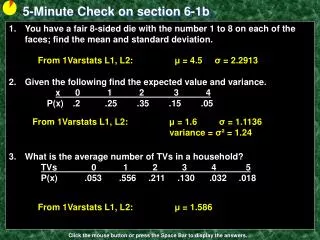
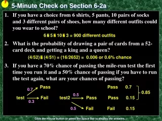
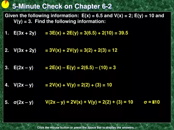
5-Minute Check on Chapter 6-2. Given the following information: E(x) = 6.5 and V(x) = 2; E(y) = 10 and V(y) = 3. Find the following information: E(3x + 2y) V(3x + 2y) E(2x – y) V(2x – y) σ(2x – y). = 3E(x) + 2E(y) = 3(6.5) + 2(10) = 39.5. = 3V(x) + 2V(y) = 3(2) + 2(3) = 12.

E N D
5-Minute Check on Chapter 6-2 • Given the following information: E(x) = 6.5 and V(x) = 2; E(y) = 10 and V(y) = 3. Find the following information: • E(3x + 2y) • V(3x + 2y) • E(2x – y) • V(2x – y) • σ(2x – y) = 3E(x) + 2E(y) = 3(6.5) + 2(10) = 39.5 = 3V(x) + 2V(y) = 3(2) + 2(3) = 12 = 2E(x) – E(y) = 2(6.5) – (10) = 3 = 2V(x) + V(y) = 2(2) + (3) = 10 V(2x – y) = 2V(x) + V(y) = 2(2) + (3) = 10 σ = 10 Click the mouse button or press the Space Bar to display the answers.
Lesson 6 - 3 Discrete Distributions Binomial and Geometric
Objectives • DETERMINE whether the conditions for a binomial setting are met • COMPUTE and INTERPRET probabilities involving binomial random variables • CALCULATE the mean and standard deviation of a binomial random variable and INTERPRET these values in context • CALCULATE probabilities involving geometric random variables
Vocabulary • Binomial Setting – random variable meets binomial conditions • Trial – each repetition of an experiment • Success – one assigned result of a binomial experiment • Failure – the other result of a binomial experiment • PDF – probability distribution function; assigns a probability to each value of X • CDF – cumulative (probability) distribution function; assigns the sum of probabilities less than or equal to X • Binomial Coefficient – combination of k success in n trials • Factorial – n! is n (n-1) (n-2) … 2 1
Discrete Probability Distributions • AP Distributions: • Uniform (seen already) • Binomial • Geometric • Non-AP Distributions: • Hypergeometric • Negative Binomial • Poisson
Criteria for a Binomial Setting A random variable is said to be a binomial provided: • The experiment is performed a fixed number of times. Each repetition is called a trial. • The trials are independent • For each trial there are two mutually exclusive (disjoint) outcomes: success or failure • The probability of success is the same for each trial of the experiment Most important skill for using binomial distributions is the ability to recognize situations to which they do and don’t apply
Acronym for Binomial RVs Definition: A binomial setting arises when we perform several independent trials of the same chance process and record the number of times that a particular outcome occurs. The four conditions for a binomial setting are • Binary? The possible outcomes of each trial can be classified as “success” or “failure.” B • Independent?Trials must be independent; that is, knowing the result of one trial must not have any effect on the result of any other trial. I N • Number?The number of trials n of the chance process must be fixed in advance. S • Success?On each trial, the probability p of success must be the same.
Example 1a Does this setting fit a binomial distribution? Explain • NFL kicker has made 80% of his field goal attempts in the past. This season he attempts 20 field goals. The attempts differ widely in distance, angle, wind and so on. Probable not binomial – probability of success would not be constant
Example 1b Does this setting fit a binomial distribution? Explain • NBA player has made 80% of his foul shots in the past. This season he takes 150 free throws. Basketball free throws are always attempted from 15 ft away with no interference from other players. Probable binomial – probability of success would be constant
Binomial Random Variable Consider tossing a coin n times. Each toss gives either heads or tails. Knowing the outcome of one toss does not change the probability of an outcome on any other toss. If we define heads as a success, then p is the probability of a head and is 0.5 on any toss. The number of heads in n tosses is a binomial random variable X. The probability distribution of X is called a binomial distribution. Definition: The count X of successes in a binomial setting is a binomial random variable. The probability distribution of X is a binomial distribution with parameters n and p, where n is the number of trials of the chance process and p is the probability of a success on any one trial. The possible values of X are the whole numbers from 0 to n.
Probability of Success • If the population is not big enough, so that the trials are not independent (usually seen with the term: without replacement), then we will have to use a Hyper-geometric Distribution (not an AP topic)
Blood Type Example Each child of a particular pair of parents has probability 0.25 of having type O blood. Genetics says that children receive genes from each of their parents independently. If these parents have 5 children, the count X of children with type O blood is a binomial random variable with n = 5 trials and probability p = 0.25 of a success on each trial. In this setting, a child with type O blood is a “success” (S) and a child with another blood type is a “failure” (F). What’s P(X = 2)? P(SSFFF) = (0.25)(0.25)(0.75)(0.75)(0.75) = (0.25)2(0.75)3 = 0.02637 However, there are a number of different arrangements in which 2 out of the 5 children have type O blood: SSFFF SFSFF SFFSF SFFFS FSSFF FSFSF FSFFS FFSSF FFSFS FFFSS Verify that in each arrangement, P(X = 2) = (0.25)2(0.75)3 = 0.02637 Therefore, P(X = 2) = 10(0.25)2(0.75)3 = 0.2637
Binomial Coefficient Note, in the previous example, any one arrangement of 2 S’s and 3 F’s had the same probability. This is true because no matter what arrangement, we’d multiply together 0.25 twice and 0.75 three times. We can generalize this for any setting in which we are interested in k successes in n trials. That is, Definition: The number of ways of arranging k successes among n observations is given by the binomial coefficient for k = 0, 1, 2, …, n where n! = n(n – 1)(n – 2)•…•(3)(2)(1) and 0! = 1.
Binomial Notation There are n independent trials of the experiment Let p denote the probability of success and then 1 – p is the probability of failure (sometimes q = 1 – p ) Let x denote the number of successes in n independent trials of the experiment. So 0 ≤ x ≤ n Determining probabilities: With your calculator: 2nd VARS 0 yields 2nd VARS A yields binompdf(n,p,x) binomcdf(n,p,x) Some Books have binomial tables, ours does not
Binomial PDF vs CDF • Abbreviation for binomial distribution is B(n,p) • A binomial pdf function gives the probability of a random variable equaling a particular value, i.e., P(x=2) • A binomial cdf function gives the probability of a random variable equaling that value or less , i.e., P(x ≤ 2) • P(x ≤ 2) = P(x=0) + P(x=1) + P(x=2)
English Phrases P(x ≤ A) = cdf (A) P(x = A) = pdf (A) P(X) ∑P(x) = 1 Cumulative probability or cdf P(x ≤ A) P(x > A) = 1 – P(x ≤ A) Values of Discrete Variable, X X=A
Binomial PDF The probability of obtaining x successes in n independent trials of a binomial experiment, where the probability of success is p, is given by: P(x) = nCx px (1 – p)n-x, x = 0, 1, 2, 3, …, n nCx is also called a binomial coefficient and is defined by combination of n items taken x at a time or where n! is n (n-1) (n-2) … 2 1 large parenthesis notation is used on the AP test n n! = -------------- k k! (n – k)!
Binomial Probability • The binomial coefficient counts the number of different ways in which k successes can be arranged among n trials. The binomial probability P(X = k) is this count multiplied by the probability of any one specific arrangement of the k successes Binomial Probability If X has the binomial distribution with n trials and probability p of success on each trial, the possible values of X are 0, 1, 2, …, n. If k is any one of these values, Number of arrangements of k successes Probability of n-k failures Probability of k successes
TI-83 Binomial Support • For P(X = k) using the calculator: 2nd VARS binompdf(n,p,k) • For P(X ≤ k) using the calculator: 2nd VARS binomcdf(n,p,k) • For P(X < k) is same as P(X k-1) • For P(X >k) use 1 – P(X k)
Example 2 In the “Pepsi Challenge” a random sample of 20 subjects are asked to try two unmarked cups of pop (Pepsi and Coke) and choose which one they prefer. If preference is based solely on chance what is the probability that: a) 6 will prefer Pepsi? b) 12 will prefer Coke? P(d=P) = 0.5 P(x) = nCx px(1-p)n-x P(x=6 [p=0.5, n=20]) = 20C6 (0.5)6(1- 0.5)20-6 = 20C6 (0.5)6(0.5)14 = 0.037 P(x=12 [p=0.5, n=20]) = 20C12 (0.5)12(1- 0.5)20-12 = 20C12 (0.5)12(0.5)8 = 0.1201
Example 2 cont P(d=P) = 0.5 P(x) = nCx px(1-p)n-x c) at least 15 will prefer Pepsi? d) at most 8 will prefer Coke? P(at least 15) = P(15) + P(16) + P(17) + P(18) + P(19) + P(20) Use cumulative PDF on calculator P(X ≥ 15) = 1 – P(X ≤ 14) = 1 – 0.9793 = 0.0207 P(at most 8) = P(0) + P(1) + P(2) + … + P(6) + P(7) + P(8) Use cumulative PDF on calculator P(X ≤ 8) = 0.2517
Example 3 A certain medical test is known to detect 90% of the people who are afflicted with disease Y. If 15 people with the disease are administered the test what is the probability that the test will show that: a) all 15 have the disease? b) at least 13 people have the disease? P(x) = nCx px(1-p)n-x P(Y) = 0.9 P(x=15 [p=0.9, n=15]) = 15C15 (0.9)15(1- 0.9)15-15 = 15C15 (0.9)15(0.1)0 = 0.20589 P(at least 13) = P(13) + P(14) + P(15) Use cumulative PDF on calculator P(X ≥ 13) = 1 – P(X ≤ 12) = 1 – 0.1841 = 0.8159
Example 3 cont P(Y) = 0.9 P(x) = nCx px(1-p)n-x c) 8 have the disease? P(x=8 [p=0.9, n=15]) = 15C8 (0.9)8(1- 0.9)15-8 = 15C8 (0.9)8(0.1)7 = 0.000277
Binomial Distribution (μB,σB) • We describe the probability distribution of a binomial random variable just like any other distribution – by looking at the shape, center, and spread. Consider the probability distribution of X = number of children with type O blood in a family with 5 children. Shape: The probability distribution of X is skewed to the right. It is more likely to have 0, 1, or 2 children with type O blood than a larger value. Center: The median number of children with type O blood is 1. Based on our formula for the mean: Spread: The variance of X is The standard deviation of X is
Binomial Mean and Std Dev • Notice, the mean µX= 1.25 can be found another way. Since each child has a 0.25 chance of inheriting type O blood, we’d expect one-fourth of the 5 children to have this blood type. That is, µX= 5(0.25) = 1.25. This method can be used to find the mean of any binomial random variable with parameters n and p. Mean and Standard Deviation of a Binomial Random Variable If a count X has the binomial distribution with number of trials n and probability of success p, the mean and standard deviation of X are Note: These formulas work ONLY for binomial distributions. They can’t be used for other distributions!
Binomial Distributions in Statistical Sampling The binomial distributions are important in statistics when we want to make inferences about the proportion p of successes in a population. Suppose 10% of CDs have defective copy-protection schemes that can harm computers. A music distributor inspects an SRS of 10 CDs from a shipment of 10,000. Let X = number of defective CDs. What is P(X = 0)? Note, this is not quite a binomial setting. Why? The actual probability is Using the binomial distribution, In practice, the binomial distribution gives a good approximation as long as we don’t sample more than 10% of the population. Sampling Without Replacement Condition When taking an SRS of size n from a population of size N, we can use a binomial distribution to model the count of successes in the sample as long as
Normal Approximation to Binomial • As n gets larger, something interesting happens to the shape of a binomial distribution. The figures below show histograms of binomial distributions for different values of n and p. What do you notice as n gets larger? Normal Approximation for Binomial Distributions Suppose that X has the binomial distribution with n trials and success probability p. When n is large, the distribution of X is approximately Normal with mean and standard deviation As a rule of thumb, we will use the Normal approximation when n is so large that np≥ 10 and n(1 – p) ≥ 10. That is, the expected number of successes and failures are both at least 10.
Normal Apx Example • Sample surveys show that fewer people enjoy shopping than in the past. A survey asked a nationwide random sample of 2500 adults if they agreed or disagreed that “I like buying new clothes, but shopping is often frustrating and time-consuming.” Suppose that exactly 60% of all adult US residents would say “Agree” if asked the same question. Let X = the number in the sample who agree. Estimate the probability that 1520 or more of the sample agree. 1) Verify that X is approximately a binomial random variable. B: Success = agree, Failure = don’t agree I: Because the population of U.S. adults is greater than 25,000, it is reasonable to assume the sampling without replacement condition is met. N: n = 2500 trials of the chance process S: The probability of selecting an adult who agrees is p = 0.60 2) Check the conditions for using a Normal approximation. Since np = 2500(0.60) = 1500 and n(1 – p) = 2500(0.40) = 1000 are both at least 10, we may use the Normal approximation.
Normal Apx Example cont • Sample surveys show that fewer people enjoy shopping than in the past. A survey asked a nationwide random sample of 2500 adults if they agreed or disagreed that “I like buying new clothes, but shopping is often frustrating and time-consuming.” Suppose that exactly 60% of all adult US residents would say “Agree” if asked the same question. Let X = the number in the sample who agree. Estimate the probability that 1520 or more of the sample agree. 3) Calculate P(X ≥ 1520) using a Normal approximation. normalcdf(1520,2500,1500,24.49) =
Summary and Homework • Summary • Binomial experiments have 4 specific criteria that must be met • Fixed number of trials • Independent trials • Two mutually exclusive outcomes • Probability of success is constant • Calculator has pdf and cdf functions • Homework • Pg 61, 65, 66, 69-77 odd
5-Minute Check on Section 6-3a What are the four conditions for a binomial experiment? Compute the probability of x successes in the n independent trials of the binomial experiment for the following values: n = 10, p = 0.7, x = 6 Compute the mean and standard deviation of the binomial random variable with the following parameters; n = 10, p = 0.7 Name the two conditions for allowing a normal approximation of a binomial random variable: Binary (success or failure) Number of trials fixed Independent trials Success probability constant P(x = 6) = E(x) = μ = (10)(0.7) = 7 σ(x) = np(1-p) = 10(.7)(.3) = 2.1 = 1.45 np ≥ 10 n(1 – p) ≥ 10 both number of successes and failures are at least 10 Click the mouse button or press the Space Bar to display the answers.
Geometric Probability Criteria An experiment is said to be a geometric experiment provided: • Each repetition is called a trial. • For each trial there are two mutually exclusive (disjoint) outcomes: success or failure • The trials are independent • The probability of success is the same for each trial of the experiment • We repeat the trials until we get a success
Geometric Settings Acronym Definition: A geometric setting arises when we perform independent trials of the same chance process and record the number of trials until a particular outcome occurs. The four conditions for a geometric setting are • Binary? The possible outcomes of each trial can be classified as “success” or “failure.” B I • Independent?Trials must be independent; that is, knowing the result of one trial must not have any effect on the result of any other trial. T • Trials?The goal is to count the number of trials until the first success occurs. S • Success?On each trial, the probability p of success must be the same.
Birthday Game The random variable of interest in this game is Y = the number of guesses it takes to correctly identify the birth day of one of your teacher’s friends. What is the probability the first student guesses correctly? The second? Third? What is the probability the kth student guesses correctly? Verify that Y is a geometric random variable. B: Success = correct guess, Failure = incorrect guess I: The result of one student’s guess has no effect on the result of any other guess. T: We’re counting the number of guesses up to and including the first correct guess. S: On each trial, the probability of a correct guess is 1/7. Calculate P(Y = 1), P(Y = 2), P(Y = 3), and P(Y = k) P(Y = 1) = 1/7 = 0.1428 P(Y = 2) = (6/7)(1/7) = 0.1224 P(Y = 3) = (6/7)(6/7)(1/7) = 0.1050 Notice the pattern?
Geometric Notation When we studied the Binomial distribution, we were only interested in the probability for a success or a failure to happen. The geometric distribution addresses the number of trials necessary before the first success. If the trials are repeated k times until the first success, we will have had k – 1 failures. If p is the probability for a success and q (1 – p) the probability for a failure, the probability for the first success to occur at the kth trial will be (where x = k) P(x) = p(1 – p)x-1, x = 1, 2, 3, … The probability that more than n trials are needed before the first success will be P(k > n) = qn= (1 – p)n
Geometric PDF The geometric distribution addresses the number of trials necessary before the first success. If the trials are repeated k times until the first success, we will have had k – 1 failures. If p is the probability for a success and q = (1 – p) the probability for a failure, the probability for the first success to occur at the kth trial will be (where x = k) P(x) = p(1 – p)x-1, x = 1, 2, 3, … even though the geometric distribution is considered discrete, the x values can theoretically go to infinity
TI-83 Geometric Support • For P(X = k) using the calculator: 2nd VARS geometpdf(p,k) • For P(k ≤ X) using the calculator: 2nd VARS geometcdf(p,k) • For P(X > k) use 1 – P(k ≤ X) or (1- p)k
Geometric PDF Mean and Std Dev Geometric experiment with probability of success p has Mean μx = 1/p Standard Deviation σx = √(1-p)/p
Birthday Game Description • The table below shows part of the probability distribution of Y. We can’t show the entire distribution because the number of trials it takes to get the first success could be an incredibly large number. Shape: The heavily right-skewed shape is characteristic of any geometric distribution. That’s because the most likely value is 1. Center: The mean of Y is µY = 7. We’d expect it to take 7 guesses to get our first success. Spread: The standard deviation of Y is σY = 6.48. If the class played the Birth Day game many times, the number of homework problems the students receive would differ from 7 by an average of 6.48.
Examples of Geometric PDF • First car arriving at a service station that needs brake work • Flipping a coin until the first tail is observed • First plane arriving at an airport that needs repair • Number of house showings before a sale is concluded • Length of time(in days) between sales of a large computer system
Example 1 The drilling records for an oil company suggest that the probability the company will hit oil in productive quantities at a certain offshore location is 0.2 . Suppose the company plans to drill a series of wells. a) What is the probability that the 4th well drilled will be productive (or the first success by the 4th)? b) What is the probability that the 7th well drilled is productive (or the first success by the 7th)? P(X) = 0.2 P(x=4) = p(1 – p)x-1 = (0.2)(0.8)4-1 = (0.2)(0.8)³ = 0.1024 P(x ≤ 4) = P(1) + P(2) + P(3) + P(4) = 0.5904 P(x=7) = p(1 – p)x-1 = (0.2)(0.8)7-1 = (0.2)(0.8)6 = 0.05243 P(x ≤ 7) = P(1) + P(2) + … + P(6) + P(7) = 0.79028
Example 1 cont The drilling records for an oil company suggest that the probability the company will hit oil in productive quantities at a certain offshore location is 0.2 . Suppose the company plans to drill a series of wells. c) Is it likely that x could be as large as 15? d) Find the mean and standard deviation of the number of wells that must be drilled before the company hits its first productive well. P(X) = 0.2 P(x) = p(1 – p)x-1 P(x=15) = p(1 – p)x-1 = (0.2)(0.8)15-1 = (0.2)(0.8)14 = 0.008796 P(x ≥ 15) = 1 - P(x ≤ 14) = 1 - 0.95602 = 0.04398 Mean: μx = 1/p = 1/0.2 = 5 (drills before a success) Standard Deviation : σx = (√1-p)/p) = (.8)/(.2) = 4 = 2
Example 2 An insurance company expects its salespersons to achieve minimum monthly sales of $50,000. Suppose that the probability that a particular salesperson sells $50,000 of insurance in any given month is .84. If the sales in any one-month period are independent of the sales in any other, what is the probability that exactly three months will elapse before the salesperson reaches the acceptable minimum monthly goal? P(X) = 0.84 P(x) = p(1 – p)x-1 P(x=3) = p(1 – p)x-1 = (0.84)(0.16)3-1 = (0.84)(0.16)2 = 0.0215
Example 3 An automobile assembly plant produces sheet metal door panels. Each panel moves on an assembly line. As the panel passes a robot, a mechanical arm will perform spot welding at different locations. Each location has a magnetic dot painted where the weld is to be made. The robot is programmed to locate the dot and perform the weld. However, experience shows that the robot is only 85% successful at locating the dot. If it cannot locate the dot, it is programmed to try again. The robot will keep trying until it finds the dot or the panel moves out of range. a) What is the probability that the robot's first success will be on attempts n = 1, 2, or 3? P(x) = p(1 – p)x-1 P(X) = 0.85 P(x=1) = p(1 – p)x-1 = (0.85)(0.15)1-1 = (0.85)(0.15)0 = 0.85 P(x=2) = p(1 – p)x-1 = (0.85)(0.15)2-1 = (0.85)(0.15)1 = 0.1275 P(x=3) = p(1 – p)x-1 = (0.85)(0.15)3-1 = (0.85)(0.15)2 = 0.019125
Example 3 cont An automobile assembly plant produces sheet metal door panels. Each panel moves on an assembly line. As the panel passes a robot, a mechanical arm will perform spot welding at different locations. Each location has a magnetic dot painted where the weld is to be made. The robot is programmed to locate the dot and perform the weld. However, experience shows that the robot is only 85% successful at locating the dot. If it cannot locate the dot, it is programmed to try again. The robot will keep trying until it finds the dot or the panel moves out of range. b) The assembly line moves so fast that the robot only has a maximum of three chances before the door panel is out of reach. What is the probability that the robot is successful in completing the weld before the panel is out of reach? P(x=1, 2, or 3) = P(1) + P(2) + P(3) = 0.996625
Example 4 In our experiment we roll a die until we get a 3 on it. a) What is the average number of times we will have to roll it until we get a 3? μx = 1/p = 1/(1/6) = 6
Example 4 cont b) What is the median number of times we will have to roll it until we get a 3? c) If they are different, then why? MDx = ∑p(xi) ≥ 0.5 = P(x=1) + P(x=2) + P(x=3) + P(x=4) = .167 + .139 + .116 + .097 = .519 μx ≥ MDx because of right skewed data
Summary and Homework • Summary • Probability of first success • Geometric Experiments have 4 slightly different criteria than Binomial • E(X) = 1/p and V(X) = (1-p)/p • Calculator has pdf and cdf functions • Homework • Pg 79-89 odd