Download
1 / 28
300 likes | 430 Views
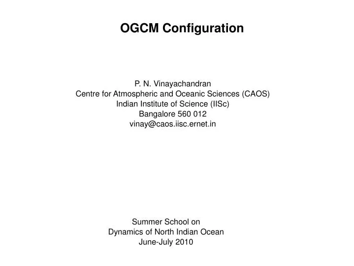
OGCM Configuration. P. N. Vinayachandran Centre for Atmospheric and Oceanic Sciences (CAOS) Indian Institute of Science (IISc) Bangalore 560 012 vinay@caos.iisc.ernet.in. Summer School on Dynamics of North Indian Ocean June-July 2010. OSCAR Currents. Equations of Motion.

E N D
OGCM Configuration P. N. Vinayachandran Centre for Atmospheric and Oceanic Sciences (CAOS) Indian Institute of Science (IISc) Bangalore 560 012 vinay@caos.iisc.ernet.in Summer School on Dynamics of North Indian Ocean June-July 2010
Spherical Co-ordinate System r=radius of the earth =latitude =longitude
Modular Ocean Model Hydrostatic Thin shell Boussinesq Sub-grid scale processes are represented by eddy mixing coefficients
Water column thickness: D = H + H(x,y) = Ocean depth; = (x,y,t) is the sea surface deviation from rest (z=0) Kinematic surface and bottome boundary conditions At z= At z=-H Griffies, 2001, MOM4 guide
Equation for free surface Ocean surface is affected by three processes: 1. Convergence of vertically integrated momentum 2. Mass entering through the ocean surface 3. Water column dialations due to changes in vertically inegrated density field (steric effects) Water column thickness: D = H + For a Boussinesq ocean: Assume volume sources/sinks only at the surface lead to balance of volume per unit area within a ocean column Kinematic surface and bottom boundary conditions At z= At z=-H = volume per unit time per unit horizontal area of freshwater crossing the sea surface = depth integrated horizontal velocity field
Surface dynamic boundary conditions for momentum and freshwater Bottom drag Closed Lateral boundaries : no slip, no normal flow Open lateral boundaries : sponge
Smagorinsky viscosity Viscosity depends on flow, nonlinear Viscosity due to unresolved scales are proportional to (deformation rates X △2) Viscosity: Deformation rate: km is the largest resolvable wave number How do you choose ? Grid Reynolds No. should be < 2 Let Then for R < 2 Tracers, Veronis effect, background viscosity Griffies, S. M.: Fundamentals of Ocean Climate Models, Princeton University Press, Princeton, USA, 518+xxxiv pages, 2004.
Horizontal Grid Size Horizontal grid spacing should resolve the Rossby Radius Rossby radius = cm/f Equatorail Rossby radius =( cm/)1/2 Eqn. 14.83 m m
Topography ETOPO5, ETOPO2 & modified Minimum depth of the ocean is 30m. Cells are deepened Isolated ocean points are converted to land Palk strait is closed, Red Sea and Persian Gulf are connected to the Arabian Sea, widened to allow 2 grid points
Sigma – coordinates (Princeton Ocean Model) Mellor, 2002
ROMS Non-linear stretching of the vertical coordinates depending on local water depth Haidvogel et al., 2000