Financial Markets and Expectations

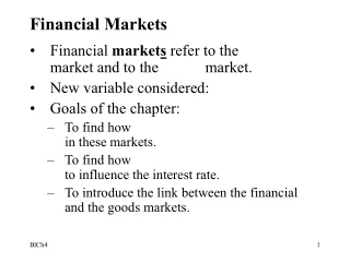
1. Financial Markets and Expectations The purpose of this lecture is two-fold: • Determination of bond prices and the Yield curve and the relationship between the Yield Curve and changes in economic conditions and macroeconomic policy; • Determination of stock prices and how fluctuations in economic conditions and macroeconomic policy may account for movements in the stock market.

2. When you considered financial markets in macroeconomics course, it was assumed that there were only two types of assets in the economy: money and a one-year bond. • Now we consider an economy which is comprised of the following financial assets: money, short-term bonds, long-term bonds and stocks. • How do expectations determine the prices of these bonds and stocks? • How does changes in monetary and fiscal policy influence the prices of bonds and stocks?

3. Lecture Outline More formally, this lecture is organized as follows: • Bonds and Yields; • The Yield Curve; • The Yield Curve and the IS/LM model; • Stock Prices; • Stock market and macroeconomic policy; • Bubbles, Fads and Stock Prices

4. Bonds and Yields • Bonds differ in two basic dimensions: • Default risk, the risk that the issuer of the bond will not pay back the full amount promised by the bond. • Bonds are typically rated according to the default risk; • Difference between the interest paid on a bond and the interest rate paid on the bond with the highest rating is called the risk premium • Bonds with high default risk are known as Junk Bonds.

5. Maturity, the length of time over which the bond promises to make payments to the holder of the bond. • Discount Bonds which promise a single payment at maturity; • Coupon Bonds that promise multiple payments before maturity and one payment at maturity.

6. Bonds of different maturities each have a price and an associated interest rate called the yield to maturity, or simply the yield. • Yields on bonds with a short maturity (less than 1 year) are called short-term interest rates. • Yields on bonds with a longer maturity are called long-term interest rates. • Yield Curve: Relationship between maturity and yield.

7. Bond market Assumptions: • Markets are forward-looking. • In equilibrium, prices must make investors equally willing to buy or sell a bond: any other price will place everyone on only one side of the market! (arbitrage condition). • Assume the Expectations Hypothesis holds, i.e we ignore the implications of risk associated with holding a particular bond. Financial investors care only about expected return.

8. Consider two types of bonds: • A one-year bond—a bond that promises one payment of $100 in one year. • A two-year bond—a bond that promises one payment of $100 in two years. • Price of the one-year bond: • Price of the two-year bond: • Price must be equal to the present value of payment of $100 next year

9. Which bond should you hold? Depends on how much you receive one year from now • Hold a 1-year bond then you receive $(1+it) next year • Hold a 2-year bond then you receive next year • Given that we are assuming that the Expectations Hypothesis holds, if investors only care about expected return, it follows that the two bonds must offer the same expected one-year return. • Why? Otherwise if the expected return was different, investors would only hold the bond with the highest expected return and the demand for the other bond would exceed supply (Thus the market for this bond cannot be in equilibrium!).

10. Expected return per dollar from holding a 2-year bond for one year. Return per dollar from holding a 1-year bond for one year. • Thus we obtain the arbitrage relation:

11. The yield to maturity on an n-year bond, or the n-year interest rate, is the constant annual interest rate that makes the bond price today equal to the present value of future payments of the bond. , then: therefore:

12. The yield to maturity on a two-year bond, is closely approximated by: Thus, the two-year interest rate is the average of the current one-year interest rate and next year’s expected one-year interest rate. • Therefore the long-term interest rate equals the average of current and future expected short-term interest rates.

13. The Yield Curve • Yield curve shows the interest rates for different maturities. • Why do we care? The slope of the yield curve tells us what financial markets expect short-term interest rates will be in the future! • Downward-sloping yield curve: • Long-term interest rates < short-term interest rates • Financial markets expect short-term interest rates to fall • Downward sloping yield curve is often taken as a signal for a forthcoming recession! • Upward-sloping yield curve: • Long-run interest rates > short-term interest rates • Financial markets expect short-term interest rates to rise

14. U.S. Yield Curves: November 1, 2000 and June 1, 2001 The yield curve, which was slightly downward sloping in November 2000, was sharply upward sloping seven months later.

15. Yield Curve and the IS/LM model • Assume that expected inflation is zero so real and nominal interest rates are the same. • Note this is to simplify the analysis: the conclusions are not affected by changing this assumption. • How can we explain the shape of the yield curve using the basic IS/LM model? • Consider a downward-sloping yield curve. • Financial markets expect an decrease in short-term rates in the future. • Why?

16. They might anticipate a slow-down in the economy brought about by a decrease in consumer confidence or future investment is expected to fall. • Thus the IS curve is expected to shift to the left and output will fall. • The financial markets thus anticipate that the monetary authority will attempt to counteract this fall in output by implementing a more expansionary monetary policy, leading to a downward-shift in the LM curve. • For both reasons therefore they expect short-term interest rates to be lower in the future, thus explaining a downward-sloping yield curve.

17. An adverse shift in spending, together with a monetary expansion, combined to lead to a decrease in the short-term interest rate.

18. Now consider an Upward-sloping Yield curve • Financial markets expect consumer confidence or investment to increase, shifting the IS curve to the right. • They also anticipate that the monetary authority may implement a more contractionary monetary policy, leading to an upward shift in the LM curve. • For both reasons therefore they expect short-term interest rates to be higher in the future, thus explaining a upward-sloping yield curve.

19. Financial markets expect stronger spending and tighter monetary policy to lead to higher short-term interest rates in the future.

20. Conclusions • The slope of the yield curve tells us what financial markets expect to happen to short-term interest rates in the future. • If financial markets expect a future monetary expansion, the expected future short-term interest rate will fall causing the yield curve to become flatter. • If a future tax cut is expected, the expected future short-term interest rate will increase causing the yield curve to become steeper. • If a future reduction in consumer confidence is expected (and thus a future reduction in consumer spending), the expected future short-term interest rate will decrease, causing the yield curve to become flatter.

21. Stock Prices • Firms raise external funds in two ways: • Through debt finance—bonds and loans; and • Through equity finance, through issues of stocks—or shares. • Bonds pay predetermined amounts; stocks pay dividends from the firm’s profits. • Dividends increase as firm’s profits increase.

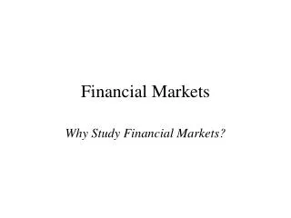
22. Standard and Poor’s Stock Price Index in Nominal and Real Terms, 1960-2000 Nominal stock prices have multiplied by 25 since 1960. Real stock prices have only multiplied by 4. Real stock prices went through a slump until the late 1980s. Only since then have they grown rapidly.

23. The price of a stock must equal the present value of future expected dividends • The nominal stock price $Qt equals the expected present discounted value of future nominal dividends $De, discounted by current and future nominal interest rates.

24. The real stock price Qt equals the expected present discounted value of future real dividends De, discounted by current and future real interest rates. • This relation has two important implications: • Higher expected future real dividends lead to a higher real stock price. • Higher current and expected future one-year real interest rates lead to a lower real stock price.

25. Changes in stock prices are essentially unpredictable. • They follow a Random Walk, i.e. price of an asset are independent over time. It is as likely to go up as it is to go down! • Note that a random walk is a sign of market efficiency. • While movements in the stock market cannot be predicted we can still use our basic IS/LM model to consider how the stock market is likely to react to changes in economic conditions and macroeconomic policy.

26. Stock market and macroeconomic policy • Again assume for simplicity that expected inflation is zero such that the real and nominal interest rates are the same. • Recall that higher future real dividends lead to a higher real stock price whereas higher future real interest rates lead to a lower real stock price. • Now consider the effect of an expansionary monetary policy. The LM curve shifts downwards, nominal interest rate falls and output increases. • How will the stock market react to this change in macroeconomic activity?

27. An Expansionary Monetary Policy and the Stock Market A monetary expansion decreases the interest rate and increases output. What it does to the stock market depends on whether financial markets anticipated the monetary expansion.

28. Expected vs Unexpected policy changes • If the policy was expected before monetary policy was changed then there should be no effect on stock prices! • Why? Expectations of future dividends and interest rates cannot be influenced by a move that has already been anticipated! • If the policy was unexpected then the stock market will react to this shock, such that stock prices should go up. • Why? Unexpected increase in output which implies higher profits and higher dividends in the short-run • Lower interest rates also implies higher stock prices

29. Source of Shocks • Now consider instead a shift in the IS curve (unexpected) • i.e. Suppose there is an unexpected increase in consumer confidence such that the IS curve shifts to the right. • This leads to higher output and higher interest rates. • Will stock prices change? • It will depend upon two key factors: • How much output and interest rates are affected • Depends on the monetary authority’s behaviour to such a shock

30. The increase in consumption spending leads to a higher interest rate and a higher level of output. What happens to the stock market depends on the slope of the LM curve and on the Fed’s behavior. An Increase in Consumption Spending and the Stock Market

31. Higher output implies higher profits and dividends (and thus higher stock prices) • Higher interest rates implies lower stock prices • Result is ambiguous: depends on the slope of the LM curve: • LM curve is steep: large increase in interest rates and a small increase in output. Thus stock prices are likely to decrease. • LM curve is flat: large increase in output and a small increase in interest rates. Thus stock prices are likely to increase.

32. An Increase in Consumption Spending and the Stock Market If the LM curve is flat, the interest rate increases little, and output increases a lot. Stock prices go up. If the LM curve is steep, the interest rate increases a lot, and output increases little.

33. Market Expectations on the Reaction of the Monetary Authority • However this result is only valid if the monetary authority does not change its policy stance. • If it is believed that the central bank will accommodate the shift in the IS curve by increasing the money supply to maintain the same level of interest rates (the LM curve shifts downwards). • Output is higher, interest rates are unchanged so stock prices should increase. • If it is believed that the monetary authority will be worried about higher inflation and tighten monetary policy, output is not affected and interest rates rise so stock prices should decrease.

34. If the Fed accommodates, the interest rate does not increase, but output does. Stock prices go up. If the Fed decides instead to keep output constant, the interest rate increases, but output does not. Stock prices go down. An Increase in Consumption Spending and the Stock Market

35. Therefore changes in macroeconomic policy and output may be associated with changes in stock prices depending upon: • The expectations of future macroeconomic policy • Source of shocks • How the market expects the monetary authority to react to changes in output.

36. Bubbles, Fads and Stock Prices • Stock prices are not always equal to their fundamental value which we defined as the present value of expected dividends. • Sometimes stocks are underpriced or overpriced. • Stock prices can be subject to bubbles or fads that lead to a stock price to differ from its fundamental value. • Bubbles occur when stocks are bought at a price higher than its fundamental value in anticipation of getting an even higher price in the future when selling. • Fads encompasses a fashion or overoptimism when stocks are bought at a higher price than the fundamental value of the stock

37. Rational speculative bubbles can occur even when investors are rational and arbitrage holds! • Stock prices may increase because investors expect them too and the bubble inflates • Even when a crash occurs those investors who hold the stock at this time (and make huge losses) where still acting rationale. While there was a chance of a crash, there was also a chance the bubble would continue. • Fads on the other-hand typically encompass irrational behaviour.

38. The general question of what determines stock prices is that bubbles and fads can play an important role as well as fundamentals. • This is important! Why? • The stock market plays a crucial role in the macro-economy. • Stock prices may react to changes in economic activity. But as we will see next week, economic activity is also influenced by the stock market! • How? Through its influence on consumption and investment decisions. • Therefore if the stock market crashes because of speculative bubbles this can have serious consequences for the real economy as consumption and investment spending can be negatively impacted.