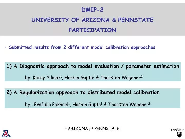
DMIP-2 UNIVERSITY OF ARIZONA & PENNSTATE PARTICIPATION

1. DMIP-2 UNIVERSITY OF ARIZONA & PENNSTATE PARTICIPATION • Submitted results from 2 different model calibration approaches • A Diagnostic approach to model evaluation / parameter estimation • by: Koray Yilmaz1, Hoshin Gupta1 & Thorsten Wagener2 • A Regularization approach to distributed model calibration • by : Prafulla Pokhrel1, Hoshin Gupta1 & Thorsten Wagener2 1 ARIZONA ; 2 PENNSTATE

2. Watershed … Blue River Basin Area 1232 sq Km Run off ratio around 0.2 Runoff ratio 0.2 Area 1232 sq km

3. PART-1 Diagnostic Evaluation of the HL-DHMS Model: A Process-based Approach

4. INFORMATION DATA CONTEXT Numbers Hyd. Theory Inferred Process Activity OBSERVABILITY & IDENTIFIABILITY of the system • Information content of the data • Efficiency in information extraction CONSISTENCY ACCURACY PRECISION Information about of the model Data .vs. Information The nature of data used: Quantity + Quality Success of model identification (calibration) depends on

5. Present Increase in computing power Increase in computing power • Increased temporal & spatial observations • Highly complex (distributed) models • Simple aggregate measures • (RMSE, Nash Sutcliffe Efficiency) Numeric measure -> guide optimization Data Flow Duration Curve Automated but Not-So-Smart “Manual” but Smart Evolution of Model Identification Approaches Past • Limited observations • Simple models • Thoughtful analysis of observations • (Flow duration curve, Budyko curve) Contextual Information!!! Signature Behavior

6. Future Present Increase the sophistication of analysis • Targeted observations (hard & soft) • Increased temporal & spatial observations • Models of various complexity • Highly complex (distributed) models • Thoughtful analysis of observations • (Flow duration curve, Budyko curve) • Simple aggregate measures • (RMSE, Nash Sutcliffe Efficiency) Contextual Information!!! Numeric measure -> guide optimization Data Signature Behavior Flow Duration Curve Automated ANDSmart (rooted in hydrologic theory ... CONTEXT) Automated but Not-So-Smart Evolution of Model Identification Approaches

7. Future Increase in sophistication of analysis • Targeted observations (hard & soft) • Increased temporal & spatial observations • Models of various complexity • Highly complex (distributed) models • Thoughtful analysis of observations • (Flow duration curve, Budyko curve) • Simple aggregate measures • (RMSE, Nash Sutcliffe Efficiency) Contextual Information!!! Numeric measure -> guide optimization Data Signature Behavior Flow Duration Curve Evolution of Model Identification Approaches Present Maximize the Likelihood that the Signature Behaviors in the Data(Info) could have been generated by the Model M Maximize the Likelihood that the DataDobs could have been generated by the Model M

8. Diagnostic Approach Extract MULTIPLE MEASURES (Information) of model support from the data The measures must be carefully designed to have DIAGNOSTIC POWER based on the HYDROLOGIC CONTEXT (Theory) -> Aggregate RESIDUAL BASED measures have poor diagnostic power ! DIAGNOSTIC EVALUATION OF MODEL is done using a MULTIPLE-CRITERIA approach CONSISTENCY is a higher goal than OPTIMALITY

9. Strategy • Assumptions that the Following are Appropriate • Conceptualization of System • HL-DHMS Structure • Koren et al (2000) strategy for A Priori Estimation (APE) of parameters • Set Up Baseline Model • Study Area (DMIP Basins / Bluo2, Eldo2, Wtto2, others) • Static Data Sets (Topography, Landcover, Soils) • Input-State-Output Data Sets (Precipitation, PET, Streamflow) • Initial Checks for Consistency • Initialization of State Variables • Corrections to I-S-O data (e.g., PET) • Corrections to A Priori Parameter Estimates (e.g., Landcover classification) • Diagnostic Evaluation of Baseline Performance • Checks on Water Balance (Time Hierarchical Approach) • Development of Diagnostic Signatures (Balance, Flow Partitioning, Timing) • Relate Parameters/Processes to Diagnostic Signatures • Sensitivity / Identifiability Analysis • Develop Method for Constraining/Adjusting Parameters • Diagnostic Multi-Criteria Evaluation Approach • Spatial Regularization • Structured Approach to Constraining Parameters • Analyze Prediction Uncertainty • Inputs, Parameter Estimates, Model Structure • Data Assimilation & Updating

10. Routing : Kinematic Hillslope & Flow Routing Channel Network Hillslopes Koren et al.,2004 Hydrologic Model • Hydrologic Model – HL-DHMS U.S. National Weather Service • Hydrology Laboratory Distributed Hydrological Modeling System Each grid : Sacramento Soil Moisture (4kmX4km) Accounting Model 16 parameters 5 states

11. MODEL PARAMETERS SOIL TEXTURE Baseline Model Setup • Based on A-priori Framework of Koren et al. (2000) • A set of physically-based relationships between 11 SAC-SMA model parameters & soil properties • Use multipliers or non linear transformation functions to adjust • a priori parameter maps

12. Evaluation of Six Year Baseline Run (10/1996 - 9/2002) Flow Duration Curve

13. VB Signature Index Partitioning SI Timing/Shape SI’s Spatial Dist SI’s Annual Hourly DiagnosingPrimary Functions of A Watershed Model Continuity Equation P ET Spatial Distribution Volume Balance Partitioning X Q Timing ROUTING SOIL MOISTURE ACCOUNTING Function Information Contained In Volume Balance - Cumulative Bias Plot Vertical Flow Partitioning - Flow Duration Curve Timing - Lag-time (Hydrograph Shape) Spatial Distribution - Along-Channel Flow Profiles

14. Diagnostic Information In Flow Duration Curve Log Flow Duration Curve Riva Volume Bias Partitioning

15. Sensitivity of Flow Duration Curve to One-at-a-time Parameter Perturbations OVERALL WATER BALANCE PARAMETER FUNCTIONING Overall Water Balance UZTWM, PFREE, LZTWM, ADIMP Flow Partitioning UZK, REXP, LZFSM, LZFPM Hydrograph Shape / Timing LZPK, LZSK, UZFWM, UZK, PCTIM, RIVA, ROUTING PARTITIONING SHAPE

16. Signature Indicator of Timing • A simple procedure to compute lag time between rainfall & its associated flow event: shift the rainfall sequence forward in time by some optimum lag that maximizes the correlation between the streamflow time series and the shifted rainfall time series. include only high flows above a threshold flow level SIM OBS Flow Threshold (mm/hr) Lag Time (hours)

17. Analysis of Parameter Sets • Parameter sets resulting in improved consistency than baseline model ±Baseline Model performance

18. Manual Calibration using Diagnostic Approach • Time hierarchical Stepwise Calibration

19. Improved Signature Match

20. PART-2 A Regularization approach to distributed model calibration

21. Model Distributed Hydrologic Model University of Arizona (DHMUA) • Water Balance component SACSMA • Routing component Muskingum Routing Method - Hill slope routing neglected

22. Model … Routing Scheme • Precipitation excess from each pixel travels instantaneously to the node • Then routing is done along the main channel (from upstream node to the downstream node)

23. Model… Parameters Input - Data Output precipitation data NEXRAD Stage III temporal scale - 1 hr Spatial scale - 16 km2 78 pixels A SACSMA – 11 distributed 5 Lumped B DHMUA O Potential Evaporation Mean monthly free surface evap. Routing - 2 parameters Lumped (Picture source http://www.nws.noaa.gov/oh/hrl/distmodel/rms.html )

24. Comparison betweenHLRMS(Hydrological Laboratory Research Modeling System) andDHMUA simulations using the apriori SACSMA parameters WY 2000 and 2001

25. Calibration

26. Proposed Hypothesis to solve high dimensional calibration Problem (REGULARIZATION APPROACH) Spatial variability of the watershed can often be well behaved and exhibit patterns (if recognized ) allows implementing some sort of constraints to reduce dimension of the parameter estimation problem. The term regularization refers to such measures, that use additional information or constraints to address ill posed or over parameterized inverse problems (Doherty and Skahill 2005).

27. Proposed Hypothesis to solve high dimensional calibration Problem (REGULARIZATION APPROACH) Koren et al. (2000) method provides A Priori Estimates of Sacramento Soil Moisture Accounting (SACSMA) (Burnash et al. 1973) parameters based on soils, topography and land cover data Info about constraints on spatial parameter variability is embedded in the A Priori Estimates, and can be used to reduce parameter dimension. (Picture source http://www.nws.noaa.gov/oh/hrl/distmodel/rms.html )

28. Development of Regularization Constraints - 1 Started with Distributed A Priori Estimates of 11 SAC-SMA Parameters based on Koren et al. (2000) Examined relationship of the A Priori Estimates to various watershed characteristics Elevation Aspect Soil depth (ZMAX) Curve number (CN) Slope X-sectional & Longitudinal curvature Vegetation type Specific catchment area Soil moisture content Topographic index Examined inter-parameter relations among the A Priori Estimates

29. Development of Regularization Constraints – 2 … Relationship of Apriori parameter Estimates to Watershed Characteristics

30. Development of Regularization Constraints – 3 … Inter-parameter Relationships

31. Development of Regularization Constraints – 4 … Regularization relationships Regularization Equations Regression equations relating the A Priori Estimates parameters to CN & ZMAX, as well as the inter-parameter relations were used to derive 11 simple regularization relations CN ZMAX

32. Development of Regularization Constraints – 5 … Comparison of Koren Apriori Parameter Estimates and Regularized Apriori Parameter Estimates WY 2001 Node 5 A Priori Regression Coefficients computed from Koren APE Node 5 Outlet

33. Development of Regularization Constraints – 6 … general form of regularization relations The regression equations have the following general form α controls the slope controls the curvature controls the intercept Calibration of parameters (, , ) for the 11 regularization equations reduces the dimension of the problem From 78 x 11 = 858unknowns To 3 x 11 =33unknowns

34. Calibration of the Regularized Model The regularization coefficients were adjusted using the MOSCEM algorithm (Multi-objective Shuffled Complex Evolution Metropolis, Vrugt et al. 2003) and Multistep Automatic Calibration (MACS)scheme (Hogue et al. 2000) Objective functions used (Mean Squared Errorand Log Mean Squared Error) Calibration Period 1 year (WY 2001)

35. Calibration Results … Combination of stage wise and simultaneous calibrations

36. Calibration Results … Hydrograph with the calibrated set of parameters

37. Calibration Results -9 Posterior Estimates of SAC-SMA Parameters Koren A Prior Regularized Posterior

38. THANK YOU !

39. References Burnash , R., R. Ferral and R. McGuire. A Generalized Streamflow Simulation System Conceptual Modeling for Digital Computers. US. Dept. of Commerce & State of Calif. 1973. Doherty, J. and Skahill, B. E., An advanced regularization methodology for use in watershed model calibration, Journal of Hydrology, 327,2005. Duan, Q., S. Sorooshian, and V.K. Gupta, Effective and Efficient Global Optimization for Conceptual Rainfall-Runoff Models, Water Resources Research, Vol. 28, No. 4, pp. 1015-1031, 1992 Gupta HV, Sorooshian S, Hogue TS, Boyle DP., Advances in Automatic Calibration of Watershed Models. In: Calibration of Watershed Models, Water Science and Application. Vol. 6. American Geophysical Union. Washington DC, 2003. Hogue, T.S., S. Sorooshian, H.V. Gupta, A. Holz, and D. Braatz, A Multi-Step Automatic Calibration Scheme (MACS) for River Forecasting Models, Journal of Hydrometeorology, Vol. 1, No. 6, pp. 524-542, 2000 Koren, V.I., Smith, M., Wang, D., Zhang, Z., Use of soil property data in the derivation of conceptual rainfall runoff model parameters, Proc. of the 15th Conf. on Hydrology, AMS, Long Beach, CA, PP 103 – 106, 2000. Vrugt, J. A., H. V. Gupta, L. A. Bastidas, W. Bouten, and S. Sorooshian, Effective and efficient algorithm formultiobjective optimization of hydrologic models, Water Resour. Res., 39(8), 1214, 2003.

40. CONCLUDING COMMENTS • Information is Data viewed in Context (hydrological theory) • Diagnostic Evaluation  techniques for effective and efficient Information Extraction • Model Developers should be required to indicate what signature measures can be used to identify/falsify proposed model components • Signature measures should be easily extractable from data (available or proposed) • Relate “Signature Match Failures” to “Model Component Failures” inherently a MC Problem • Model Consistency a higher goal than optimality

41. SUMMARY Data is not information Information is data viewed in context Use “Information” (not data) to constrain model and diagnose deficiencies Design “Signature” Measures that relate to model functions / processes This leads to the possibility of improving our understanding and models

42. ONGOING RESEARCH Focus on: • Signature Measures to diagnose spatial variation in processes / model components • Test Signature Measures during independent evaluation periods • Test Diagnostic Model Evaluation strategy in a variety of basins

43. A-priori Framework– Koren et al. (2000, 2003) Based on soil physics: USDA Textural Triangle Cosby et al. 1984 WRR Clapp and Hornberger 1978 WRR CN Koren et al. 2003 AGU Monograph http://dbwww.essc.psu.edu/dbtop/ doc/statsgo/meth_fract.html

44. Constraining the Model Parameters • A priori Parameters as a Constraint MODEL PARAMETER • Assume spatial pattern of model parameters are • well-defined by a-priori framework • (soil properties) • Vary MULTIPLIERS within a range, so that model parameters are physically meaningful Blue River

45. Parameter Perturbations using Random Sampling (1600 parameter sets) Sensitivity of Flow Bias Parameters that control the ET Not sensitive Sensitive

46. Signature Indicator of Timing Shift in Flow Centroid (for rising and falling limbs)

47. One-at-a-time Parameter Perturbations -Sensitivity of Rising Flow Centroid O Baseline vs. Observed flows Parameter Perturbations vs. Observed flows Controls Surface flow Controls Routing