Describing Data: Displaying and Exploring Data

1. Describing Data: Displaying and Exploring Data Chapter 4 Modified by Boris Velikson, fall 2009

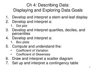
2. GOALS • Develop and interpret a dot plot. • Develop and interpret a stem-and-leaf display. • Compute and understand quartiles, deciles, and percentiles. • Construct and interpret box plots. • Compute and understand the coefficient of skewness. • Draw and interpret a scatter diagram. • Construct and interpret a contingency table.

3. Reminder: usefulness of Visual Display of Data • We showed in Chapter 2 that one can see the data at a glance if one transforms it into a Frequency Distribution. The Data: 15.0, 23.7, 19.7, 15.4, 18.3, 23.0, 14.2, 20.8, 13.5, 20.7, 17.4, 18.6, 12.9, 20.3, 13.7, 21.4, 18.3, 29.8, 17.1, 18.9, 10.3, 26.1, 15.7, 14.0, 17.8, 33.8, 23.2, 12.9, 27.1, 16.6. get transformed into afrequency distribution: And then into a histogram: At each step, we lose some information but gain in visibility.

4. Dot Plots (Dot Scale Diagrams) • A dot plot groups the data as little as possible.The identity of an individual observation is not lost. • Each observation is simply displayed as a dot along a horizontal line indicating the possible values of the data. • If there are identical observations or the observations are too close to be shown individually, the dots are “piled” on top of each other. • Dot plots are useful for comparing two or more data sets. • Dot plots can be used only for discrete data. • The usefulness of a dot plot depends on the nature of the data set.

5. Dot Plots - Examples Reported below are the number of vehicles sold in the last 24 months at Smith Ford Mercury Jeep, Inc., in Kane, Pennsylvania, and Brophy Honda Volkswagen in Greenville, Ohio. Construct dot plots and report summary statistics for the two small-town Auto USA lots. (Excel file on CDROM: Data Files – Excel and Minitab \ Chp4 \ Dotplots.xls)

6. Dot Plot – PhStat results Dot Plots cannot be produced directly by Excel. Theoretically they can be produced by MegaStat, but it often fails. This one was produced by PHStat that you do not have. So you must do it by hand.

7. Dot Plot – Minitab results (you can’t do this unless you install Minitab!) I am showing you these results despite the fact that you do not have Minitab (most probably), to show the comparison between two dot plots.

8. WARNING about Dot Plots • You do not have MiniTab (it is not free), not PhStat (you get it with a different book). • On some computers, MegaStat does not work well when you try to obtain Dot Plots with it. (You can try it on Dotplot.xls, figuring among Chapter 4 Excel files) • Therefore, you draw them by hand. • This is not so bad: anyway, Dot Plots are useful only for small sets of data.

9. Stem-and-Leaf • In Chapter 2, frequency distribution was used to organize data into a meaningful form. • A major advantage to organizing the data into a frequency distribution is that we get a quick visual picture of the shape of the distribution. • There are two disadvantages, however, to organizing the data into a frequency distribution: • The exact identity of each value is lost • Difficult to tell how the values within each class are distributed. • One technique that is used to display quantitative information in a condensed form is the stem-and-leaf display.

10. Stem-and-Leaf • Stem-and-leaf display is a statistical technique to present a set of data. Each numerical value is divided into two parts. The leading digit(s) becomes the stem and the trailing digit the leaf. The stems are located along the vertical axis, and the leaf values are stacked against each other along the horizontal axis. • Advantage of the stem-and-leaf display over a frequency distribution - the identity of each observation is not lost. This means that we have the data: 88,89,93,94,94,95,96,96,97,…,155,155,156 We choose the stem size so that each class is reasonably populated. For these data, the stem size is 10. It may only be a power of 10 (0.1, 1, 10, 100…)

11. Stem-and-Leaf Plot Example Let’s do this example in more detail. (The data are in the file Table4-1.xls) Listed in Table 4–1 is the number of 30-second radio advertising spots purchased by each of the 45 members of the Greater Buffalo Automobile Dealers Association last year. Organize the data into a stem-and-leaf display. Around what values do the number of advertising spots tend to cluster? What is the fewest number of spots purchased by a dealer? The largest number purchased?

12. Stem-and-Leaf Plot Example There are two possibilities: doing all the work by hand or using MegaStat (because you do not have MiniTab). However, MegaStat often fails to produce a stem-and-leaf plot (an error is produced). So let’s do it by hand. • Decide on the stem value. Here the data spans from 88 to 156, and there are no fractional data. It does not make sense to have a stem size of 1 (then most lines will be empty) or 100 (then the plot will have only two lines). The stem size is, therefore, 10. • Prepare the stems (from 8 to 15). • Go over the data, splitting each into the stem and the leaf: for example, 86 will have a stem of 8 and a leaf of 6, and 148, a stem of 14, and a leaf of 4. Mark each leaf on the corresponding stem line. • Sort the leafs on each line in the increasing order.

13. Stem-and-Leaf Plot Example The result is

14. Stem-and-Leaf – Another Example Stock prices on twelve consecutive days for a major publicly traded company: 86,79,92,84,69,88,91,83,96,78,82,85.

15. In-Class Exercises and Homework (dot plots and steam-and-leaf plots) • In class: P. 105 No. 3, 5, 7, 9 • Homework: No. 4, 6, 8, 10

16. Quartiles, Deciles and Percentiles • The most widely used measure of dispersion is the standard deviation. • Another frequently used way of describing spread of data is determining the location (sequential number in the set)of values that divide a set of observations into equal parts. • We already had one such measure: the median divides a set of observation in two parts. • These measures include quartiles (which divide the set in four parts), deciles (in ten parts), and percentiles (in 100 parts).

17. Quartiles - Example Listed below are the commissions earned last month by a sample of 15 brokers at Salomon Smith Barney’s Oakland, California, office. Salomon Smith Barney is an investment company with offices located throughout the United States. $2038 $1758 $1721 $1637 $2097 $2047 $2205 $1787 $2287 $1940 $2311 $2054 $2406 $1471 $1460 .

18. Quartiles– Example (cont.) Step 1: Organize the data from lowest to largest value median The middle value (the median) location is found by Lmed = (15+1)/2 = 8. There are 7 values below the median and 7 values above. Because the median divides the data into two halves, we also call it the 50th percentile (P50) and we say that it is located at L50. In our case, L50=Lmed= 8, and P50=median=$2038.

19. Quartiles– Example (cont.) Step 2: Compute the first and third quartiles. Locate L25 and L75 using: Therefore, the first and the fourth quartile are the 4th and the 12th observation in the array:

20. Quartiles – Example (cont.) Step 2: Compute the first and third quartiles. median 3d quartile 1st quartile In a similar way, we can split the values in 4 parts. The values separating the 4 parts are called quartiles. The 1st quartile is located at the position L25=(n+1)/4=(n+1)(25/100). Here, L25=(15+1)/4=4. The value of the 1st quartile is Q1 =$1721. The 3d quartile is located at the position L75=(n+1)(3/4) =(n+1)(75/100).Here, L75=(15+1)(3/4)=12. The value of the 3d quartile is Q3=$2205.

21. Percentiles Percentiles: median 3d quartile 1st quartile We also call the 1st quartile the 25th percentile, and the 3d quartile, the 75th percentile. (Then we write P25 instead of Q1, and P75 instead of Q3). In general,

22. Percentiles – Example (cont.) What if the number of data can’t be divided by 4? Suppose we have 12 observations in a sample. Then But there is no observation no. 3.25 or 9.75! So what do we do? We take the 3d and the 4th observations X3 and X4, and form a value which is ¼-way between the two. This will be Q1. Then we take X9 and X10 and form a value which is ¾ way between the two. This will be Q3.

23. Percentiles – Example (cont.) 50th percentile: Median Price at 6.50th observation = 84 + .5(85-84) = 84.50 25th percentile: 1st quartile Price at 3.25th observation = 79 + .25(82-79) = 79.75 75th percentile: 3d quartile Price at 9.75th observation = 88 + .75(91-88) = 90.25

24. Deciles; Percentiles other than Quartiles We call deciles percentiles that are multiples of 10. L10 is the location of the first decile, L30 of the 3d decile, etc. We will call the value of the first decile D1 (this is the same as P10) etc.

25. Percentiles – Example (Excel Data Analysis) Read p.109

26. Percentiles – Example (MegaStat)

27. Interquartile Range The Interquartile range is the distance between the third quartile Q3 and the first quartile Q1. This distance will include the middle 50 percent of the observations. Interquartile range = Q3 - Q1 Here Q1 and Q3 are the values of the quartiles.

28. Boxplot - Example

29. Boxplot Example Step1: Create an appropriate scale along the horizontal axis. Step 2: Draw a box that starts at Q1 (15 minutes) and ends at Q3 (22 minutes). Inside the box we place a vertical line to represent the median (18 minutes). Step 3: Extend horizontal lines from the box out to the minimum value (13 minutes) and the maximum value (30 minutes).

30. Boxplot – Using MegaStat Develop a box plot of the data for the data below from Chapter 2. What can we conclude about the distribution of the vehicle selling prices?

31. Boxplot – Using MegaStat What can we conclude about the distribution of the vehicle selling prices? • Conclude: • The median vehicle selling price is about $23,000, • About 25 percent of the vehicles sell for less than $20,000, and that about 25 percent sell for more than $26,000. • About 50 percent of the vehicles sell for between $20,000 and $26,000. • The distribution is positively skewed because the solid line above $26,000 is somewhat longer than the line below $20,000.

32. Outliers Outliers are the data that lie more than 1.5 times the interquartile distance on the left of Q1 or on the right of Q3. In this example, Q1=$20000, Q3=$26000. So an outlier would be 1.5×6000=9000 away, i.e. less than 20000-9000=$11000 or more than 26000+9000=$35000. We see an asterisk marking an outlier. In a MiniTab output, the upper whisker extends only to the non-outlier maximum ($32492), and the two outliers are represented by asterisk. In a MegaStat output, outliers are not marked, and the upper whisker extends to the maximum value. Be prepared to interpret different kinds of outputs. Attn.: different authors may define outliers in a slightly different way (not necessarily exactly 1.5 times the interquartile distance away)

33. In-Class Exercises and Homework (boxplots) • In class: P. 113-114 No. 15, 17 • Homework: No. 16,18 • In doing the box plot exercises, let’s stick to the following convention if you produce a box plot by hand: • The whiskers run to the maximum or minimum value or to 1.5 times the interquartile distance from the box ends, whichever is closer to the box. • The outliers are values that lie outside these values.

34. Skewness • In Chapter 3, measures of central location (the mean, median, and mode) for a set of observations and measures of data dispersion (e.g. range and the standard deviation) were introduced • Another characteristic of a set of data is the shape. • There are four shapes commonly observed: • symmetric, • positively skewed, • negatively skewed, • bimodal.

35. Skewness - Formulas for Computing The coefficient of skewness can range from -3 up to 3. • A value near -3, indicates considerable negative skewness. • A value such as 1.63 indicates moderate positive skewness. • A value of 0, which will occur when the mean and median are equal, indicates the distribution is symmetrical and that there is no skewness present. (in fact, the software coefficient works better, but if you have only a simple calculator, it is easier to calculate Pearson’s)

36. Commonly Observed Shapes

37. Skewness – An Excel Example • Following are the earnings per share for a sample of 15 software companies for the year 2007. The earnings per share are arranged from smallest to largest. • Compute the mean, median, and standard deviation. Find the coefficient of skewness using both Pearson’s and software estimates. • What is your conclusion regarding the shape of the distribution?

38. Skewness – An Excel Example This is a clickable Excel file,you can see the formulas if you open it.

39. Skewness – A MegaStat Example This is a MegaStat output. The skewness obtained here is the software coefficient of skewness.

40. Commonly Observed Shapes

41. Describing Relationship between Two Variables • When we study the relationship between two variables we refer to the data as bivariate. • One graphical technique we use to show the relationship between variables is called a scatter diagram. • To draw a scatter diagram we need two variables. We scale one variable along the horizontal axis (X-axis) of a graph and the other variable along the vertical axis (Y-axis).

42. In-Class Exercises and Homework (skewness) • In class: P. 117 No. 19 • Homework: No. 22

43. Describing Relationship between Two Variables • One graphical technique we use to show the relationship between variables is called a scatter diagram. • To draw a scatter diagram we need two variables. We scale one variable along the horizontal axis (X-axis) of a graph and the other variable along the vertical axis (Y-axis).

44. Describing Relationship between Two Variables – Scatter Diagram Examples

45. Describing Relationship between Two Variables – Scatter Diagram Excel Example In Chapter 2 we presented data from AutoUSA. In this case the information concerned the prices of 80 vehicles sold last month at the Whitner Autoplex lot in Raytown, Missouri. The data shown include the selling price of the vehicle as well as the age of the purchaser. Is there a relationship between the selling price of a vehicle and the age of the purchaser? Would it be reasonable to conclude that the more expensive vehicles are purchased by older buyers?

46. Describing Relationship between Two Variables – Scatter Diagram Excel Example

47. Contingency Tables • A scatter diagram requires that both of the variables be at least interval scale. • What if we wish to study the relationship between two variables when one or both are nominal or ordinal scale? In this case we tally the results in a contingency table.

48. Contingency Tables A contingency table is a cross-tabulation that simultaneously summarizes two variables of interest. Examples: • Students at a university are classified by gender and class rank. • A product is classified as acceptable or unacceptable and by the shift (day, afternoon, or night) on which it is manufactured. • A voter in a school bond referendum is classified as to party affiliation (Democrat, Republican, other) and the number of children that voter has attending school in the district (0, 1, 2, etc.).

49. Contingency Tables – An Example A manufacturer of preassembled windows produced 50 windows yesterday. This morning the quality assurance inspector reviewed each window for all quality aspects. Each was classified as acceptable or unacceptable and by the shift on which it was produced. Thus we reported two variables on a single item. The two variables are shift and quality. The results are reported in the following table. Using the contingency table able, the quality of the three shifts can be compared. For example: On the day shift, 3 out of 20 windows or 15 percent are defective. On the afternoon shift, 2 of 15 or 13 percent are defective and On the night shift 1 out of 15 or 7 percent are defective. Overall 12 percent of the windows are defective

50. More Homework • Homework: No. 37,42,43