The Visibility Problem

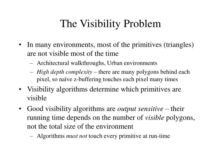
1. The Visibility Problem • In many environments, most of the primitives (triangles) are not visible most of the time • Architectural walkthroughs, Urban environments • High depth complexity – there are many polygons behind each pixel, so naïve z-buffering touches each pixel many times • Visibility algorithms determine which primitives are visible • Good visibility algorithms are output sensitive – their running time depends on the number of visible polygons, not the total size of the environment • Algorithms must not touch every primitive at run-time

2. Visibility Algorithm Taxonomy • Back-face culling: remove polygons with normals facing away from the viewer • For closed objects, such faces must be occluded by the front of the object • View frustum culling: remove polygons that fall outside the viewing frustum • Exact visibility: locate the set of polygons that are at least partially visible, and no others • Approximate visibility: locate most of the visible polygons and only a few of the non-visible ones • Conservative visibility: locate all of the partially visible polygons, and maybe some others

3. Minimalist Approach • Perform view volume culling in software • Break the world into some hierarchical data structure (Octree, BSP) • Associate objects/polygons with leaves of the tree • Start at the root • Send the contents of cells completely within the view frustum to the rendering pipeline • Ignore cells completely outside the view frustum • Recurse into children of cells straddling the view frustum • Back-face culling is implemented in hardware for render • Culled polygons reach the clipping stage of the pipeline • Assuming a roughly uniform scene, and a 45° FOV, this will send 1/8th of the scene to the graphics pipeline, and 1/16th of the scene to the rasterizer

4. Exact Visibility • Computes the set of polygons that are visible, and no others • Difficult, with provably high worst case complexity. How high? • Their use is limited to non-walkthrough applications: • Shadow rendering, where we care about which surfaces are visible from the light source • Form factor computations for radiosity • Visibility is required from every patch to every other patch • It is worth building large data structures to make visibility efficient • Computer vision: View space partitioning and aspect graphs

5. Conservative Visibility • Producing a slightly larger potentially visible set (PVS) is generally much easier than producing the exact set • Send all the PVS to the graphics pipeline and let the z-buffer sort out the exact set • Z-buffer hardware remains efficient provided each pixel is not over-rendered many times – so the PVS cannot be too large • Almost all practical visibility algorithms are conservative and generate a PVS • A further primary distinguishing feature: • Object-space algorithms do their computations in world space • Image space algorithms project objects or bounds into image space before determining visibility

6. Cells and Portals(Airey 90, Teller and Sequin 91, Luebke and Georges 95) • Best in architectural scenes • Cells are rooms • Portals are doorways and windows • The boundaries of the cells (the walls) block almost everything, so visibility is reduced very quickly without the need to merge occluders • Cells are generally built using a BSP tree • Walls (large polygons) suggest good splitting planes • Try to keep the tree balanced, while cutting as few polygons as possible (because cut polygons are associated with both cells) • Ignore the detail objects (furniture) • Portals are gaps in cell boundaries

7. Cells and Portals (cont) • As a preprocess, associate a PVS with every cell • Set of all other cells visible from some point inside this cell • Note that all PV cells must be visible from somewhere on a portal • Several ways to build the set • Shadow volumes (normally used for area light sources) • Random sampling of rays • Linear programming to find stabbing lines in 2d • A stabbing line connects PV cells through a sequence of portals • Each portal provides two constraints to the linear program • Use depth first search to find all stabbing lines • Specialized algorithms find stabbing lines in 3d • Operate in the dual space (find stabbing “points” in line space)

8. Cells and Portals (cont) • Simplest algorithm renders all the PVS for the current cell • Includes cells behind the viewer, as well as other invisible cells • Instead, traverse the stab-tree and crop the view frustum to each portal • Don’t render cells that do not lie inside the cropped view frustum • Preprocessing PVS is actually unnecessary • Start with view frustum in current cell • Crop to each portal out of the cell • Recurse on neighboring cells with cropped frustum • Doesn’t tell you which cells may be required soon, so they cannot be paged from disk ahead of time • The BEST visibility scheme for densely occluded interiors that fit into memory (mazes in computer games)

9. Large Occluders but No Cells(Coorg and Teller 97) • Many scenes are not easily broken into cells with small portals • Several new ideas • Choose the occluders at run-time, from a pre-computed set of possibilities • Cull kd-tree cells against the chosen occluders • Fast culling by noting the existence of separating planes and supporting planes Partially Occluded Occluded Partially Occluded Supporting Separating Fully visible

10. Choosing Occluders • Good occluders cover large areas of the image • Large in size • Close to the viewer • Aligned front on • Associate a set of occluders with each leaf of the kd-tree • Use set for the cell that contains the viewer • Combine occluders that share a non-silhouette edge • Ignore supporting planes through common edge • Cache supporting planes for subsequent frames Area A N V D eye

11. Other Object-Space Algorithms • Coorg and Teller also describe an alternate algorithm: • Explicitly construct the set of separating planes for views local the the current one • Identifies when those planes are invalidated and builds new ones • Effectively computes and maintains a subset of the linearized aspect graph • The Visibility Skeleton (Durand, Drettakis, Puech 1997) • Computes a full subset of the aspect graph • Used for radiosity form factor computations – makes it easy to identify discontinuity lines and compute exact visibility • Other theoretical approaches: The visibility complex(Durand, Drettakis, Puech 1996), and the asp (Plantinga and Dyer 1990)