Download
1 / 27
380 likes | 1.29k Views
Finite Sample Properties of the Least Squares Estimator. Based on Greene’s Lecture Note 6 . Terms of Art. Estimates and estimators Properties of an estimator - the sampling distribution “Finite sample” properties as opposed to “asymptotic” or “large sample” properties.

E N D
Finite Sample Properties of the Least Squares Estimator Based on Greene’s Lecture Note 6
Terms of Art • Estimates and estimators • Properties of an estimator - the sampling distribution • “Finite sample” properties as opposed to “asymptotic” or “large sample” properties
The Statistical Context of Least Squares Estimation The sample of data from the population: (y,X) The stochastic specification of the regression model: y = Xb + e Endowment of the stochastic properties of the model upon the least squares estimator
Deriving the Properties So, b = a parameter vector + a linear combination of the disturbances, each times a vector. Therefore, b is a vector of random variables. We analyze it as such. The assumption of nonstochastic regressors. How it is used at this point. We do the analysis conditional on an X, then show that results do not depend on the particular X in hand, so the result must be general – i.e., independent of X.
Properties of the LS Estimator Expected value and the property of unbiasedness. E[b|X] = = E[b]. Prove this result. A Crucial Result About Specification: y = X11 + X22 + Two sets of variables. What if the regression is computed without the second set of variables? What is the expectation of the "short" regression estimator? b1 = (X1X1)-1X1y
The Left Out Variable Formula E[b1] = 1 + (X1X1)-1X1X22 The (truly) short regression estimator is biased. Application: Quantity = 1Price + 2Income + If you regress Quantity on Price and leave out Income. What do you get? (Application below)
The Extra Variable Formula A Second Crucial Result About Specification: • y = X11 + X22 + but 2 really is 0. Two sets of variables. One is superfluous. What if the regression is computed with it anyway? The Extra Variable Formula: E[b1.2| 2 = 0] = 1 The long regression estimator in a short regression is unbiased.) Extra variables in a model do not induce biases. Why not just include them, then? We'll pursue this later.
Application: Left out Variable Leave out Income. What do you get? E[b1] = 1 + 2 In time series data, 1 < 0, 2 > 0 (usually) Cov[Price,Income] > 0 in time series data. So, the short regression will overestimate the price coefficient. Simple Regression of G on a constant and PG Price Coefficient should be negative.
Estimated ‘Demand’ Equation • Simple Regression of G on a constant and PG. Price Coefficient should be negative? • Multiple Regression of G on a constant, PG, and Y. • Multiple Regression of G on a constant, PG, Y and extra variables: PNC, PUC.
Gauss-Markov Theorem Gauss and Markov Theorem: Least Squares is the BLUE (or MVLUE) • Linear estimator • Unbiased: E[b|X] = β • Minimum varianceComparing positive definite matrices: Var[c|X] – Var[b|X] is nonnegative definite for any other linear and unbiased estimator. What are the implications?
Aspects of the Gauss-Markov Theorem Indirect proof: Any other linear unbiased estimator has a larger covariance matrix. Direct proof: Find the minimum variance linear unbiased estimator Other estimators Biased estimation – a minimum mean squared error estimator. Is there a biased estimator with a smaller ‘dispersion’? Normally distributed disturbances – the Rao-Blackwell result. (General observation – for normally distributed disturbances, ‘linear’ is superfluous.) Nonnormal disturbances - Least Absolute Deviations and other nonparametric approaches
Fixed X or Conditioned on X? The role of the assumption of nonstochastic regressors Finite sample results: Conditional vs. unconditional results Its importance in the asymptotic results.
Specification Errors-1 Omitting relevant variables: Suppose the correct model is y = X11 + X22 + . I.e., two sets of variables. Compute least squares omitting X2. Some easily proved results: Var[b1] is smaller than Var[b1.2]. (The latter is the northwest submatrix of the full covariance matrix. The proof uses the residual maker (again!). I.e., you get a smaller variance when you omit X2. (One interpretation: Omitting X2 amounts to using extra information (2 = 0). Even if the information is wrong (see the next result), it reduces the variance. (This is an important result.)
Omitted Variables (No free lunch) E[b1] = 1 + (X1X1)-1X1X221. So, b1 is biased.(!!!) The bias can be huge. Can reverse the sign of a price coefficient in a “demand equation.” b1 may be more “precise.” Precision = Mean squared error = variance + squared bias. Smaller variance but positive bias. If bias is small, may still favor the short regression. (Free lunch?) Suppose X1X2 = 0. Then the bias goes away. Interpretation, the information is not “right,” it is irrelevant. b1 is the same as b1.2.
Specification Errors-2 Including superfluous variables: Just reverse the results. Including superfluous variables increases variance. (The cost of not using information.) Does not cause a bias, because if the variables in X2 are truly superfluous, then 2 = 0, so E[b1.2] = 1.
Linear Least Squares Subject to Restrictions Restrictions: Theory imposes certain restrictions on parameters. Some common applications Dropping variables from the equation = certain coefficients in b forced to equal 0. (Probably the most common testing situation. “Is a certain variable significant?”) Adding up conditions: Sums of certain coefficients must equal fixed values. Adding up conditions in demand systems. Constant returns to scale in production functions. Equality restrictions: Certain coefficients must equal other coefficients. Using real vs. nominal variables in equations. Common formulation: Minimize the sum of squares, ee, subject to the linear constraint Rb = q.
Aspects of Restricted LS 1. b* = b - Cm where m = the “discrepancy vector” Rb - q. Note what happens if m = 0. What does m = 0 mean? 2. =[R(XX)-1R]-1(Rb - q) = [R(XX)-1R]-1m. When does = 0. What does this mean? 3. Combining results: b* = b - (XX)-1R. How could b* = b?
Linear Restrictions Context: How do linear restrictions affect the properties of the least squares estimator? Model: y = X + Theory (information) R - q = 0 Restricted least squares estimator: b* = b - (XX)-1R[R(XX)-1R]-1(Rb - q) Expected value: - (XX)-1R[R(XX)-1R]-1(Rb - q) Variance: 2(XX)-1 - 2 (XX)-1R[R(XX)-1R]-1R(XX)-1 Var[b] – a nonnegative definite matrix < Var[b]
Interpretation Case 1: Theory is correct: R - q = 0 (the restrictions do hold). b* is unbiased Var[b*] is smaller than Var[b] How do we know this? Case 2: Theory is incorrect: R - q 0 (the restrictions do not hold). b* is biased – what does this mean? Var[b*] is still smaller than Var[b]
Restrictions and Information How do we interpret this important result? The theory is "information" Bad information leads us away from "the truth" Any information, good or bad, makes us more certain of our answer. In this context, any information reduces variance. What about ignoring the information? Not using the correct information does not lead us away from "the truth" Not using the information foregoes the variance reduction - i.e., does not use the ability to reduce "uncertainty."
Example • Linear Regression Model: y = Xb + eG = b0 + b1PG + b2Y + b3PNC + b4PUC + ey = G; X = [1 PG Y PNC PUC] • Linear Restrictions: Rb – q = 0b3 = b4 = 0