Download
1 / 37
370 likes | 502 Views
Motion Estimation using Markov Random Fields. Hrvoje Bogunović Image Processing Group Faculty of Electrical Engineering and Computing University of Zagreb Summer School on Image Processing, Graz 2004. Overview. Introduction Optical flow M arkov Random Fields OF+MRF combined

E N D
Motion Estimation using Markov Random Fields Hrvoje Bogunović Image Processing Group Faculty of Electrical Engineering and Computing University of Zagreb Summer School on Image Processing, Graz 2004
Overview • Introduction • Optical flow • Markov Random Fields • OF+MRF combined • Energy minimization techniques • Results
Introduction • Input: • Sequence of images (Video) • Problem • Extract information about motion • Applications • Detection, Segmentation, Tracking, Coding
Motion – aliasing Large area flicker f 1/t φ 1/x Loss of spatial resolution
Large motions - temporal aliasing f Temporal aliasing φ Great loss of spatial resolution
Temporalanti-aliasing f φ • No more overlaping on the f axis. • filtering (anit-aliasing) is performed after sampling, hence the blurring
Motion estimation • Images are 2-D projections of the 3-D world. • Problem is represented as a labeling one. • Assign vector to pixel • Vector field field of movement • Low level vision • No interpretation
Problems • Problem is inherently ill-posed • Solution is not unique • Aperture problem • Specific to local methods
Optical flow • Main assumption: Intensity of the object does not change as it moves • Often violated • First solved by Horn & Schunk • Gradient approach • Other approaches include • Frequency based • Using corresponding features
Gradient approach • Local by nature. Aperture problem is significant. • Image understanding is not required • Very low level
Horn & Schunk • Intensity stays the same in the direction of movement. I(x,y,t) •After derivation
Horn & Schunk • Spatial gradients Ix,Iy • e.g. Sobel operator • Temporal gradient It • Image subtraction
Regularization • Tikhonov regularization for ill-posed problems • Add the smoothness term • Energy function
Problems of the H-S method • Assumption: There are no discontinuities in the image • Optical flow is over-smoothed. • Gradient method. Only the edges which are perpendicular to motion vector contribute • Image regions which are uniform do not contribute. • Difficulty with large motions (spatial filtering)
Optical flow enhancement • Optical flow can be piecewise smooth • Discontinuities can be incorporated • Solution: use the spatial context • Problem is posed as a solution of the Bayes classifier. Solution in optimization sense. Search for optimum
Bayes classifier • Main equation • Solution using MAP estimation
Markov Random Fields • Suitable: Problems posed as a visual labeling problemn with contextual constraints • Useful to encode a priori knowledge • required for bayes classifier (smoothness prior) • equvalence to Gibbs random fields (gibbs distribution, exponential like) • Neighbourhoods • Cliques • pairs,triples of neighbourhood points) • build the energy function
MRF • Define sites: rectangular lattice • Define labels • define neighbourhood: 4,8 point • Field is MRF: • P(f)>0 • P(fi|f{S-i})=P(fi|Ni)
Coupled MRF • Field F is an optical flow field • Field L is a field of discontinuities • line process • Position of the two fields.
Context • neighbourhoods and cliques
Energy for MAP estimation Parameters are estimatedad hoc
Energy minimization • Global minimum • Simulated annealing • Genetic Algorithms • Local minimum • Iterated Conditional Modes (ICM) (steepest decent) • Highest Confidence First (HCF) • specific site visiting
Simulatedannealing • (1) Findthe initial temperatureof the system T. • Assign initial values of the field to random • For every pixel: • Assign random valueto f(i,j) • Calculate the difference in energy before and after If the change is better (diff>0) keep it. Else keep it with the probability exp(diff/T) • (4) Repeat (3) N1 times • (5) T = f(T) where f decreases monotono • (6) Repeat (3-5) N2 times
Results (Square) OF+MRF Horn-Schunk OF