Download
1 / 26
360 likes | 570 Views
Matrix-Vector Multiplication by MapReduce. From Rajaraman / Ullman- Ch.2 Part 1. Google implementation of MapReduce. created to execute very large matrix-vector multiplications When ranking of Web pages that goes on at search engines, n is in the tens of billions.

E N D
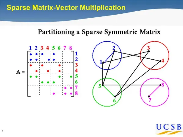
Matrix-Vector Multiplication by MapReduce From Rajaraman / Ullman- Ch.2 Part 1
Google implementation of MapReduce • created to execute very large matrix-vector multiplications • When ranking of Web pages that goes on at search engines, n is in the tens of billions. • Page Rank- iterative algorithm • Also, useful for simple (memory-based) recommender systems
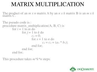
Problem Statement • Given, • n × n matrix M, whose element in row i and column j will be denoted . • a vector v of length n. • = . • Assume that • the row-column coordinates of each matrix element will be discoverable, either from its position in the file, or because it is stored with explicit coordinates, as a triple (i, j, ). • the position of element in the vector v will be discoverable in the analogous way.
Case 1: n is large, but not so large that vector v cannot fit in main memory • The Map Function: • Map function is written to apply to one element of M • v is first read to computing node executing a Map task and is available for all applications of the Map function at this compute node. • Each Map task will operate on a chunk of the matrix M. • From each matrix element it produces the key-value pair (i, ( . ) ). • Thus, all terms of the sum that make up the component of the matrix-vector product will get the same key, i.
Case 1 Continued … • The Reduce Function: • The Reduce function simply sums all the values associated with a given key i. • The result will be a pair (i, ).
Case 2: n is large to fit into main memory • v should be stored in computing nodes used for the Map task • Divide the matrix into vertical stripes of equal width and divide the vector into an equal number of horizontal stripes, of the same height. • Our goal is to use enough stripes so that the portion of the vector in one stripe can fit conveniently into main memory at a compute node.
Matrix M vector v Figure 2.4: Division of a matrix and vector into five stripes • The ith stripe of the matrix multiplies only components from the ith stripe of the vector. • Divide the matrix into one file for each stripe, and do the same for the vector. • Each Map task is assigned a chunk from one of the stripes of the matrix and gets the entire • corresponding stripe of the vector. • The Map and Reduce tasks can then act exactly as was described, as case 1.
Recommender is one of the most popular large-scale machine learning techniques. • Amazon • eBay • Facebook • Netflix • …
Two types of recommender techniques • Collaborative Filtering • Content Based Recommendation • Collaborative Filtering • Model based • Memory based • User similarity based • Item similarity based
Item-based collaborative filtering • Basic idea: • Use the similarity between items (and not users) to make predictions • Example: • Look for items that are similar to Item5 • Take Alice's ratings for these items to predict the rating for Item5
Making predictions • A common prediction function: • u –> user; i,p -> items; user has not rated item p. • Neighborhood size is typically also limited to a specific size • Not all neighbors are taken into account for the prediction • An analysis of the MovieLens dataset indicates that "in most real-world situations, a neighborhood of 20 to 50 neighbors seems reasonable" (Herlocker et al. 2002)
Pre-processing for item-based filtering • Item-based filtering does not solve the scalability problem itself • Pre-processing approach by Amazon.com (in 2003) • Calculate all pair-wise item similarities in advance • The neighborhood to be used at run-time is typically rather small, because only items are taken into account which the user has rated • Item similarities are supposed to be more stable than user similarities • Memory requirements • Up to N2 pair-wise similarities to be memorized (N = number of items) in theory • In practice, this is significantly lower (items with no co-ratings) • Further reductions possible • Minimum threshold for co-ratings • Limit the neighborhood size (might affect recommendation accuracy)
Mahout’s Item-Based RS • Apache Mahout is an open source Apache Foundation project for scalable machine learning. • Mahout uses Map-Reduce paradigm for scalable recommendation
Mahout’s RS Matrix Multiplication for Preference Prediction 1 2 3 4 5 1 2 3 4 5 1 2 3 4 5 Item-Item Similarity Matrix Active User’s Preference Vector
As matrix math, again • Inside-out method 5 5 2
Page Rank Algorithm • One iteration of the PageRank algorithm involves taking an estimated Page-Rank vector v and computing the next estimate v′ by v′ = βMv + (1 − β)e/n • β is a constant slightly less than 1, e is a vector of all 1’s, and • n is the number of nodes in the graph that transition matrix M represents.
Vectors v and v’ are too large for Main Memory • If using the stripe method to partition a matrix and vector that do not fit in main memory, then a vertical stripe from the matrix M and a horizontal stripe from the vector v will contribute to all components of the result vector v’. • Since that vector is the same length as v, it will not fit in main memory either. • M is stored column-by-column for efficiency reasons, a column can affect any of the components of v’. As a result, it is unlikely that when we need to add a term to some component , that component will already be in main memory. • Thrashing
Square Blocks, instead of Slices • An additional constraint is that the result vector should be partitioned in the same way as the input vector, so the output may become the input for another iteration of the matrix-vector multiplication. • An alternative strategy is based on partitioning the matrix into blocks, while the vectors are still partitioned into k stripes.
Iterative Computation- Square Blocks Method • In this method, we use Map tasks. Each task gets one square of the matrix M, say , and one stripe of the vector v, which must be . Notice that each stripe of the vector is sent to k different Map tasks; is sent to the task handling for each of the k possible values of i. Thus, v is transmitted over the network k times. However, each piece of the matrix is sent only once. • The advantage of this approach is that we can keep both the jth stripe of v and the ith stripe of v’ in main memory as we process . Note that all terms generated from and contribute to and no other stripe of v’.
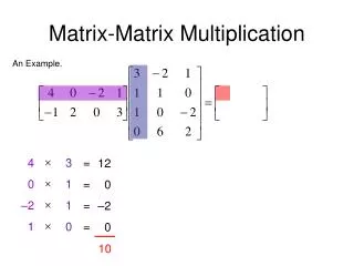
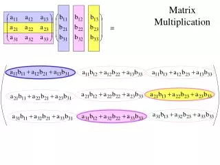
Matrix-Matrix Multiplication using MapReduce • Like Natural Join Operation
Matrix A represents a typical user-product-rating model • The algorithm tries to derive a set of latent factors (like tastes) from the user-product-rating matrix from matrix A. • So matrix X can be viewed as user-taste matrix And matrix Y can be viewed as a product-taste matrix
Objective Function • Only check observed ratings • If we fix X, the objective function becomes a convex. Then we can calculate the gradient to find Y • If we fix Y, we can calculate the gradient to find X
Iterative Training Algorithm • Given Y, you can Solve X Xi = A(T)-1 • The algorithm works in the following way: Y0 -> X1 -> Y1 -> X2 -> Y2 -> … Till the squared difference is small enough