Download
1 / 34
340 likes | 750 Views
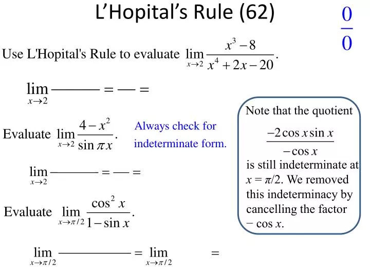
L’Hopital’s Rule (62). Note that the quotient. is still indeterminate at x = π /2. We removed this indeterminacy by cancelling the factor − cos x . Step 1. Integrate over a finite interval [2, R ]. Improper Integrals (63). Step 2. Compute the limit as R → ∞. Improper Integrals (63).

E N D
L’Hopital’s Rule (62) Note that the quotient is still indeterminate at x = π/2. We removed this indeterminacy by cancelling the factor − cosx.
Step 1.Integrate over a finite interval [2, R]. Improper Integrals (63) Step 2.Compute the limit as R → ∞.
The integral is improper because the integrand has an infinite discontinuity at x = 0. Improper Integrals (63)
(64) Deer Population A deer population grows logistically with growth constant k = 0.4 year−1 in a forest with a carrying capacity of 1000 deer. (a) Find the deer population P(t) if the initial population is P0 = 100. (b) How long does it take for the deer population to reach 500? `
Finding the Constants Partial Fractions (65)
Finding the Constants Partial Fractions (65)
Finding the Constants Partial Fractions (65)
THEOREM 2 Vector-Valued Derivatives Are Computed ComponentwiseA vector-valued function r(t) = x (t), y (t) is differentiable iff each component is differentiable. In this case, Velocity & Acceleration Vectors (66) Calculate r”(3), where r(t) = ln t, t .
The Derivative as a Tangent Vector (66) Plotting Tangent Vectors Plot r (t) = cost, sin t together with its tangent vectors at and . Find a parametrization of the tangent line at . and thus the tangent line is parametrized by
A particle travels along the path c (t) = (2t, 1 + t3/2). Find: (a) The particle’s speed at t = 1 (assume units of meters and minutes). Parametric Speed (68)
Parametric Equations: Given a Velocity Vector, Find the Position Vector (69)
Use Theorem 1 to compute the area of the right semicircle with equation r = 4 sin θ. The equation r = 4 sin θdefines a circle of radius 2 tangent to the x-axis at the origin. The right semicircle is “swept out” as θ varies from 0 to Area Inside the Polar Curve (72) By THM 1, the area of the right semicircle is
Sketch r = sin 3θand compute the area of one “petal.” Area Inside the Polar Curve (72) r varies from 0 to 1 and back to 0 as θ varies from 0 to r varies from 0 to -1 and back to 0 as θ varies from r varies from 0 to 1 and back to 0 as θ varies from
Find an equation of the line tangent to the polar curve r= sin 2θwhen
Euler’s Method (74) Let y (t) be the solution of Use Euler’s Method with time step h = 0.1 to approximate y (0.5).
Let y (t) be the solution of Use Euler’s Method with time step h = 0.1 to approximate y (0.5). When h = 0.1, yk is an approximation to y (0 + k (0.1)) = y (0.1k),so y5 is an approximation to y (0.5). It is convenient to organize calculations in the following table. Note that the value yk+1 computed in the last column of each line is used in the next line to continue the process. c c c c c c c c c c c c c c c c c c c c c c c c c c c c c c c c c c c c c Thus, Euler’s Method yields the approximation y (0.5) ≈ y5 ≈ 0.1. Is this an overestimate or underestimate? Scatter Plot is concave up!
(76) Integration by Parts applies to definite integrals:
Shortcuts to Finding Taylor Series Write a Series for… (77) There are several methods for generating new Taylor series from known ones. First of all, we can differentiate and integrate Taylor series term by term within its interval of convergence, by Theorem 2 of Section 11.6. We can also multiply two Taylor series or substitute one Taylor series into another (we omit the proofs of these facts). Find the Maclaurin series for f (x) = x2ex.
The sum of the reciprocal powers n−p is called a p-series. THEOREM 3 Convergence of p-Series The infinite series Convergence of a Geometric Series (79) converges if p > 1 and diverges otherwise. Here are two examples of p-series: