Download
1 / 75
830 likes | 1.36k Views
Spatial Statistics. Concepts (O&U Ch. 3) Centrographic Statistics (O&U Ch. 4 p. 77-81) single, summary measures of a spatial distribution Point Pattern Analysis (O&U Ch 4 p. 81-114) -- pattern analysis; points have no magnitude (“no variable”) Quadrat Analysis

E N D
Spatial Statistics Concepts (O&U Ch. 3) Centrographic Statistics (O&U Ch. 4 p. 77-81) single, summary measures of a spatial distribution Point Pattern Analysis (O&U Ch 4 p. 81-114) -- pattern analysis; points have no magnitude (“no variable”) Quadrat Analysis Nearest Neighbor Analysis Spatial Autocorrelation (O&U Ch 7 pp. 180-205 One variable The Weights Matrix Join Count Statistic Moran’s I (O&U pp 196-201) Geary’s C Ratio (O&U pp 201) General G LISA Correlation and Regression Two variables Standard Spatial Briggs UT-Dallas GISC 6382 Spring 2007
Description versus Inference • Description and descriptive statistics • Concerned with obtaining summary measures to describe a set of data • Inference and inferential statistics • Concerned with making inferences from samples about populations • Concerned with making legitimate inferences about underlying processes from observed patterns We will be looking at both! Briggs UT-Dallas GISC 6382 Spring 2007
Formulae for mean Formulae for variance å n 2 å 2 ( X X ) n å X [( X ) / N ] - 2 i - i = = = 1 i i 1 N N Classic Descriptive Statistics: UnivariateMeasures of Central Tendency and Dispersion • Central Tendency: single summary measure for one variable: • mean (average) • median (middle value) • mode (most frequently occurring) • Dispersion: measure of spread or variability • Variance • Standard deviation (square root of variance) These may be obtained in ArcGIS by: --opening a table, right clicking on column heading, and selecting Statistics --going to ArcToolbox>Analysis>Statistics>Summary Statistics Briggs UT-Dallas GISC 6382 Spring 2007
2.5% 2.5% -1.96 1.96 0 Classic Descriptive Statistics: UnivariateFrequency distributions A counting of the frequency with which values occur on a variable • Most easily understood for a categorical variable (e.g. ethnicity) • For a continuous variable, frequency can be: • calculated by dividing the variable into categories or “bins” (e.g income groups) • represented by the proportion of the area under a frequency curve In ArcGIS, you may obtain frequency counts on a categorical variable via: --ArcToolbox>Analysis>Statistics>Frequency Briggs UT-Dallas GISC 6382 Spring 2007
å n 2 ( Y Y ) Sy= å - i n - - ( x X )( y Y ) = 1 i i i = N = i 1 r n S S å n 2 ( X X ) x y SX= - i = i 1 N Classic Descriptive Statistics: BivariatePearson Product Moment Correlation Coefficient (r) • Measures the degree of association or strength of the relationship between two continuous variables • Varies on a scale from –1 thru 0 to +1 -1 implies perfect negative association • As values on one variable rise, those on the other fall (price and quantity purchased) 0 implies no association +1 implies perfect positive association • As values rise on one they also rise on the other (house price and income of occupants) Where Sx and Sy are the standard deviations of X and Y, and X and Y are the means. Briggs UT-Dallas GISC 6382 Spring 2007
Classic Descriptive Statistics: BivariateCalculation Formulae for Pearson Product Moment Correlation Coefficient (r) Correlation Coefficient example using “calculation formulae” As we explore spatial statistics, we will see many analogies to the mean, the variance, and the correlation coefficient, and their various formulae There is an example of calculation later in this presentation. Briggs UT-Dallas GISC 6382 Spring 2007
Inferential Statistics: Are differences real? • Frequently, we lack data for an entire population (all possible occurrences) so most measures (statistics) are estimated based on sample data • Statistics are measures calculated from samples which are estimates of population parameters • the question must always be asked if an observed difference (say between two statistics) could have arisen due to chance associated with the sampling process, or reflects a real difference in the underlying population(s) • Answers to this question involve the concepts of statistical inference and statistical hypothesis testing • Although we do not have time to go into this in detail, it is always important to explore before any firm conclusions are drawn. • However, never forget: statistical significance does not always equate to scientific (or substantive) significance • With a big enough sample size (and data sets are often large in GIS), statistical significance is often easily achievable • See O&U pp 108-109 for more detail Briggs UT-Dallas GISC 6382 Spring 2007
2.5% 2.5% -1.96 0 1.96 Statistical Hypothesis Testing: Classic Approach Statistical hypothesis testing usually involves 2 values; don’t confuse them! • A measure(s) or index(s) derived from samples (e.g. the mean center or the Nearest Neighbor Index) • We may have two sample measures (e.g. one for males and another for females), or a single sample measure which we compare to “spatial randomness” • A test statistic, derived from the measure or index, whose probability distribution is known when repeated samples are made, • this is used to test the statistical significance of the measure/index We proceed from the null hypothesis (Ho ) that, in the population, there is “no difference” between the two sample statistics, or from spatial randomness* • If the test statistic we obtain is very unlikely to have occurred (less than 5% chance) if the null hypothesis was true, the null hypothesis is rejected If the test statistic is beyond +/- 1.96 (assuming a Normal distribution), we reject the null hypothesis (of no difference) and assume a statistically significant difference at at least the 0.05 significance level. *O’Sullivan and Unwin use the term IRP/CSR: independent random process/complete spatial randomness Briggs UT-Dallas GISC 6382 Spring 2007
Statistical Hypothesis Testing: Simulation Approach • Because of the complexity inherent in spatial processes, it is sometime difficult to derive a legitimate test statistic whose probability distribution is known • An alternative approach is to use the computer to simulate multiple random spatial patterns (or samples)--say 100, the spatial statistic (e.g. NNI or LISA) is calculated for each, and then displayed as a frequency distribution. • This simulated sampling distribution can then be used to assess the probability of obtaining our observed value for the Index if the pattern had been random. Our observed value: --highly unlikely to have occurred if the process was random --conclude that process is not random Empirical frequency distribution from 499 random patterns (“samples”) This approach is used in Anselin’s GeoDA software
Is it Spatially Random?Tougher than it looks to decide! • Fact: It is observed that about twice as many people sit catty/corner rather than opposite at tables in a restaurant • Conclusion: psychological preference for nearness • In actuality: an outcome to be expected from a random process: two ways to sit opposite, but four ways to sit catty/corner From O’Sullivan and Unwin p.69 Briggs UT-Dallas GISC 6382 Spring 2007
Why Processes differ from Random Processes differ from random in two fundamental ways • Variation in the receptiveness of the study area to receive a point • Diseases cluster because people cluster (e.g. cancer) • Cancer cases cluster ‘cos chemical plants cluster • First order effect • Interdependence of the points themselves • Diseases cluster ‘cos people catch them from others who have the disease (colds) • Second order effects In practice, it is very difficult to disentangle these two effects merely by the analysis of spatial data Briggs UT-Dallas GISC 6382 Spring 2007
What do we mean by spatially random? UNIFORM/ DISPERSED CLUSTERED • Types of Distributions • Random: any point is equally likely to occur at any location, and the position of any point is not affected by the position of any other point. • Uniform: every point is as far from all of its neighbors as possible: “unlikely to be close” • Clustered: many points are concentrated close together, and there are large areas that contain very few, if any, points: “unlikely to be distant” RANDOM
Centrographic Statistics • Basic descriptors for spatial point distributions (O&U pp 77-81) Measures of CentralityMeasures of Dispersion • Mean Center -- Standard Distance • Centroid -- Standard Deviational Ellipse • Weighted mean center • Center of Minimum Distance • Two dimensional (spatial) equivalents of standard descriptive statistics for a single-variable distribution • May be applied to polygons by first obtaining the centroid of each polygon • Best used in a comparative context to compare one distribution (say in 1990, or for males) with another (say in 2000, or for females) This is a repeat of material from GIS Fundamentals. To save time, we will not go over it again here.Go to Slide # 25 Briggs UT-Dallas GISC 6382 Spring 2007
Mean Center • Simply the mean of the X and the Y coordinates for a set of points • Also called center of gravity or centroid • Sum of differences between the mean X and all other X is zero (same for Y) • Minimizes sum of squared distances between itself and all points Distant points have large effect. Provides a single point summary measure for the location of distribution. Briggs UT-Dallas GISC 6382 Spring 2007
Centroid • The equivalent for polygons of the mean center for a point distribution • The center of gravity or balancing point of a polygon • if polygon is composed of straight line segments between nodes, centroid again given “average X, average Y” of nodes • Calculation sometimes approximated as center of bounding box • Not good • By calculating the centroids for a set of polygons can apply Centrographic Statistics to polygons Briggs UT-Dallas GISC 6382 Spring 2007
Weighted Mean Center • Produced by weighting each X and Y coordinate by another variable (Wi) • Centroids derived from polygons can be weighted by any characteristic of the polygon Briggs UT-Dallas GISC 6382 Spring 2007
4,7 7,7 10 10 4,7 7,7 7,3 2,3 5 5 6,2 0 0 10 10 5 5 7,3 2,3 6,2 0 0 Calculating the centroid of a polygon or the mean center of a set of points. (same example data as for area of polygon) Calculating the weighted mean center. Note how it is pulled toward the high weight point. Briggs UT-Dallas GISC 6382 Spring 2007
Center of Minimum Distance or Median Center • Also called point of minimum aggregate travel • That point (MD) which minimizessum of distances between itself and all other points (i) • No direct solution. Can only be derived by approximation • Not a determinate solution. Multiple points may meet this criteria—see next bullet. • Same as Median center: • Intersection of two orthogonal lines (at right angles to each other), such that each line has half of the points to its left and half to its right • Because the orientation of the axis for these lines is arbitrary, multiple points may meet this criteria. Source: Neft, 1966 Briggs UT-Dallas GISC 6382 Spring 2007
Median and Mean Centers for US Population Median Center: Intersection of a north/south and an east/west line drawn so half of population lives above and half below the e/w line, and half lives to the left and half to the right of the n/s line Mean Center: Balancing point of a weightless map, if equal weights placed on it at the residence of every person on census day. Source: US Statistical Abstract 2003 Briggs UT-Dallas GISC 6382 Spring 2007
Formulae for standard deviation of single variable Standard Distance Deviation • Represents the standard deviation of the distance of each point from the mean center • Is the two dimensional equivalent of standard deviation for a single variable • Given by: which by Pythagorasreduces to: ---essentially the average distance of points from the center Provides a single unit measure of the spread or dispersion of a distribution. We can also calculate a weighted standard distance analogous to the weighted mean center. Or, with weights Briggs UT-Dallas GISC 6382 Spring 2007
4,7 7,7 10 7,3 2,3 5 6,2 0 10 5 0 Standard Distance Deviation Example Circle with radii=SDD=2.9 Briggs UT-Dallas GISC 6382 Spring 2007
Standard Deviational Ellipse: concept • Standard distance deviation is a good single measure of the dispersion of the incidents around the mean center, but it does not capture any directional bias • doesn’t capturethe shape of the distribution. • The standard deviation ellipse gives dispersion in two dimensions • Defined by 3 parameters • Angle of rotation • Dispersion along major axis • Dispersion along minor axis The major axis defines the direction of maximum spreadof the distribution The minor axis is perpendicular to itand defines the minimum spread Briggs UT-Dallas GISC 6382 Spring 2007
Standard Deviational Ellipse: calculation • Formulae for calculation may be found in references cited at end. For example • Lee and Wong pp. 48-49 • Levine, Chapter 4, pp.125-128 • Basic concept is to: • Find the axis going through maximum dispersion (thus derive angle of rotation) • Calculate standard deviation of the points along this axis (thus derive the length (radii) of major axis) • Calculate standard deviation of points along the axis perpendicular to major axis (thus derive the length (radii) of minor axis) Briggs UT-Dallas GISC 6382 Spring 2007
Mean Center & Standard Deviational Ellipse: example There appears to be no major difference between the location of the software and the telecommunications industry in North Texas. Briggs UT-Dallas GISC 6382 Spring 2007
Point Pattern Analysis Analysis of spatial properties of the entire body of points rather than the derivation of single summary measures Two primary approaches: • Point Densityapproach using Quadrat Analysis based on observing the frequency distribution or density of points within a set of grid squares. • Variance/mean ratio approach • Frequency distribution comparison approach • Point interactionapproach using Nearest Neighbor Analysis based on distances of points one from another Although the above would suggest that the first approach examines first order effects and the second approach examines second order effects, in practice the two cannot be separated. See O&U pp. 81-88 Briggs UT-Dallas GISC 6382 Spring 2007
Exhaustive census --used for secondary (e.g census) data Random sampling --useful in field work Frequency counts by Quadrat would be: Multiple ways to create quadrats --and results can differ accordingly! Quadrats don’t have to be square --and their size has a big influence Briggs UT-Dallas GISC 6382 Spring 2007
2 * A P Quadrat Analysis: Variance/Mean Ratio (VMR) Where: A = area of region P = # of points • Apply uniform or random grid over area (A) with width of square given by: • Treat each cell as an observation and count the number of points within it, to create the variable X • Calculate variance and mean of X, and create the variance to mean ratio: variance / mean • For an uniform distribution, the variance is zero. • Therefore, we expect a variance-mean ratio close to 0 • For a random distribution, the variance and mean are the same. • Therefore, we expect a variance-mean ratio around 1 • For a clustered distribution, the variance is relatively large • Therefore, we expect a variance-mean ratio above 1 See following slide for example. See O&U p 98-100 for another example Briggs UT-Dallas GISC 6382 Spring 2007
x x x UNIFORM/ DISPERSED CLUSTERED random uniform Clustered Formulae for variance 2 RANDOM Note: N = number of Quadrats = 10 Ratio = Variance/mean Briggs UT-Dallas GISC 6382 Spring 2007
= Significance Test for VMR • A significance test can be conducted based upon the chi-square frequency • The test statistic is given by: (sum of squared differences)/Mean • The test will ascertain if a pattern is significantly more clustered than would be expected by chance (but does not test for a uniformity) • The values of the test statistics in our cases would be: • For degrees of freedom: N - 1 = 10 - 1 = 9, the value of chi-square at the 1% level is 21.666. • Thus, there is only a 1% chance of obtaining a value of 21.666 or greater if the points had been allocated randomly. Since our test statistic for the clustered pattern is 80, we conclude that there is (considerably) less than a 1% chance that the clustered pattern could have resulted from a random process clustered 200-(202)/10=80 2 random 60-(202)/10=10 2 uniform 40-(202)/10=0 2 (See O&U p 98-100) Briggs UT-Dallas GISC 6382 Spring 2007
Quadrat Analysis: Frequency Distribution Comparison • Rather than base conclusion on variance/mean ratio, we can compare observed frequencies in the quadrats (Q= number of quadrats) with expected frequencies that would be generated by • a random process (modeled by the Poisson frequency distribution) • a clustered process (e.g. one cell with P points, Q-1 cells with 0 points) • a uniform process (e.g. each cell has P/Q points) • The standard Kolmogorov-Smirnov test for comparing two frequency distributions can then be applied – see next slide • See Lee and Wong pp. 62-68 for another example and further discussion. Briggs UT-Dallas GISC 6382 Spring 2007
Kolmogorov-Smirnov (K-S) Test • The test statistic “D” is simply given by: D = max [ Cum Obser. Freq – Cum Expect. Freq] The largest difference (irrespective of sign) between observed cumulative frequency and expected cumulative frequency • The critical value at the 5% level is given by: D (at 5%) = 1.36where Q is the number of quadrats Q • Expected frequencies for a random spatial distribution are derived from the Poisson frequency distribution and can be calculated with: p(0) = e-λ= 1 / (2.71828P/Q) and p(x) = p(x - 1) * λ/x Where x = number of points in a quadrat and p(x) = the probability of x points P = total number of points Q = number of quadrats λ = P/Q (the average number of points per quadrat) See next slide for worked example for cluster case
Row 10 The spreadsheet spatstat.xls contains worked examples for the Uniform/ Clustered/ Random data previously used, as well as for Lee and Wong’s data
Weakness of Quadrat Analysis • Results may depend on quadrat size and orientation (Modifiable areal unit problem) • test different sizes (or orientations) to determine the effects of each test on the results • Is a measure of dispersion, and not really pattern, because it is based primarily on the density of points, and not their arrangement in relation to one another • Results in a single measure for the entire distribution, so variations within the region are not recognized (could have clustering locally in some areas, but not overall) For example, quadrat analysis cannot distinguish between these two, obviously different, patterns For example, overall pattern here is dispersed, but there are some local clusters Briggs UT-Dallas GISC 6382 Spring 2007
Nearest-Neighbor Index (NNI) (O&U p. 100) • uses distances between points as its basis. • Compares the mean of the distance observed between each point and its nearest neighbor with the expected mean distance that would occur if the distribution were random: NNI=Observed Aver. Dist / Expected Aver. Dist For random pattern, NNI = 1 For clustered pattern, NNI = 0 For dispersed pattern, NNI = 2.149 • We can calculate a Z statistic to test if observedpattern is significantly different from random: • Z = Av. Dist Obs - Av. Dist. Exp. Standard Error if Z is below –1.96 or above +1.96, we are 95% confident that the distribution is not randomly distributed. (If the observed pattern was random, there are less than 5 chances in 100 we would have observed a z value this large.) (in the example that follows, the fact that the NNI for uniform is 1.96 is coincidence!)
(Standard error) Nearest Neighbor Formulae Index Where: Significance test Briggs UT-Dallas GISC 6382 Spring 2007
Mean distance Mean distance Mean distance NNI NNI NNI RANDOM CLUSTERED UNIFORM Z = 5.508 Z = -0.1515 Z = 5.855 Source: Lembro
Evaluating the Nearest Neighbor Index • Advantages • NNI takes into account distance • No quadrat size problem to be concerned with • However, NNI not as good as might appear • Index highly dependent on the boundary for the area • its size and its shape (perimeter) • Fundamentally based on only the mean distance • Doesn’t incorporate local variations (could have clustering locally in some areas, but not overall) • Based on point location only and doesn’t incorporate magnitude of phenomena at that point • An “adjustment for edge effects” available but does not solve all the problems • Some alternatives to the NNI are the G and F functions, based on the entire frequency distribution of nearest neighbor distances, and the K function based on all interpoint distances. • See O and U pp. 89-95 for more detail. • Note: the G Function and the General/Local G statistic (to be discussed later) are related but not identical to each other Briggs UT-Dallas GISC 6382 Spring 2007
Spatial Autocorrelation The instantiation of Tobler’s first law of geography Everything is related to everything else, but near things are more related than distant things. Correlation of a variable with itself through space. The correlation between an observation’s value on a variable and the value of close-by observations on the same variable The degree to which characteristics at one location are similar (or dissimilar) to those nearby. Measure of the extent to which the occurrence of an event in an areal unit constrains, or makes more probable, the occurrence of a similar event in a neighboring areal unit. Several measures available: Join Count Statistic Moran’s I Geary’s C ratio General (Getis-Ord) G Anselin’s Local Index of Spatial Autocorrelation (LISA) These measures may be “global” or “local”
Spatial Autocorrelation Positive: similar values cluster together on a map Auto: self Correlation: degree of relative correspondence Source: Dr Dan Griffith, with modification Negative: dissimilar values cluster together on a map Briggs UT-Dallas GISC 6382 Spring 2007
Why Spatial Autocorrelation Matters • Spatial autocorrelation is of interest in its own right because it suggests the operation of a spatial process • Additionally, most statistical analyses are based on the assumption that the values of observations in each sample are independent of one another • Positive spatial autocorrelation violates this, because samples taken from nearby areas are related to each other and are not independent • In ordinary least squares regression (OLS), for example, the correlation coefficients will be biased and their precision exaggerated • Bias implies correlation coefficients may be higher than they really are • They are biased because the areas with higher concentrations of events will have a greater impact on the model estimate • Exaggerated precision (lower standard error) implies they are more likely to be found “statistically significant” • they will overestimate precision because, since events tend to be concentrated, there are actually a fewer number of independent observations than is being assumed. Briggs UT-Dallas GISC 6382 Spring 2007
Measuring Relative Spatial Location • How do we measure the relative location or distance apart of the points or polygons? Seems obvious but its not! • Calculation of Wij, the spatial weights matrix, indexing the relative location of all points i and j, is the big issuefor all spatial autocorrelation measures • Different methods of calculation potentially result in different values for the measures of autocorrelation and different conclusions from statistical significance tests on these measures • Weights based on Contiguity • If zone j is adjacent to zone i, the interaction receives a weight of 1, otherwise it receives a weight of 0 and is essentially excluded • But what constitutes contiguity? Not as easy as it seems! • Weights based on Distance • Uses a measure of the actual distance between points or between polygon centroids • But what measure, and distance to what points -- All? Some? • Often, GIS is used to calculate the spatial weights matrix, which is then inserted into other software for the statistical calculations Briggs UT-Dallas GISC 6382 Spring 2007
X Weights Based on Contiguity For Regular Polygons rook case or queen case For Irregular polygons • All polygons that share a common border • All polygons that share a common border or have a centroid within the circle defined by the average distance to (or the “convex hull” for) centroids of polygons that share a common border For points • The closest point (nearest neighbor) --select the contiguity criteria --construct n x n weights matrix with 1 if contiguous, 0 otherwise An archive of contiguity matrices for US states and counties is at: http://sal.uiuc.edu/weights/index.html(note: the .gal format is weird!!!) Briggs UT-Dallas GISC 6382 Spring 2007
Weights based on Lagged Contiguity • We can also use adjacency matrices which are based on lagged adjacency • Base contiguity measures on “next nearest” neighbor, not on immediate neighbor • In fact, can define a range of contiguity matrices: • 1st nearest, 2nd nearest, 3rd nearest, etc. Briggs UT-Dallas GISC 6382 Spring 2007
Queens Case Full Contiguity Matrix for US States • 0s omitted for clarity • Column headings (same as rows) omitted for clarity • Principal diagonal has 0s (blanks) • Can be very large, thus inefficient to use.
Queens Case Sparse Contiguity Matrix for US States • Ncount is the number of neighbors for each state • Max is 8 (Missouri and Tennessee) • Sum of Ncount is 218 • Number of common borders (joins) • ncount / 2 = 109 • N1, N2… FIPS codes for neighbors
Weights Based on Distance(see O&U p 202) • Most common choice is the inverse (reciprocal) of the distance between locations i and j (wij = 1/dij) • Linear distance? • Distance through a network? • Other functional forms may be equally valid, such as inverse of squared distance (wij =1/dij2), or negative exponential (e-d or e-d2) • Can use length of shared boundary: wij= length (ij)/length(i) • Inclusion of distance to all points may make it impossible to solve necessary equations, or may not make theoretical sense (effects may only be ‘local’) • Include distance to only the “nth” nearest neighbors • Include distances to locations only within a buffer distance • For polygons, distances usually measured centroid to centroid, but • could be measured from perimeter of one to centroid of other • For irregular polygons, could be measured between the two closest boundary points (an adjustment is then necessary for contiguous polygons since distance for these would be zero) Briggs UT-Dallas GISC 6382 Spring 2007
A Note on Sampling Assumptions • Another factor which influences results from these tests is the assumption made regarding the type of sampling involved: • Free (or normality) sampling assumes that the probability of a polygon having a particular value is not affected by the number or arrangement of the polygons • Analogous to sampling with replacement • Non-free (or randomization) sampling assumes that the probability of a polygon having a particular value is affected by the number or arrangement of the polygons (or points), usually because there is only a fixed number of polygons (e.g. if n = 20, once I have sampling 19, the 20th is determined) • Analogous to sampling without replacement • The formulae used to calculate the various statistics (particularly the standard deviation/standard error) differ depending on which assumption is made • Generally, the formulae are substantially more complex for randomization sampling—unfortunately, it is also the more common situation! • Usually, assuming normality sampling requires knowledge about larger trends from outside the region or access to additional information within the region in order to estimate parameters.
Joins (or joint or join) Count Statistic • For binary (1,0) data only (or ratio data converted to binary) • Shown here as B/W (black/white) • Requires a contiguity matrix for polygons • Based upon the proportion of “joins” between categories e.g. • Total of 60 for Rook Case • Total of 110 for Queen Case • The “no correlation” case is simply generated by tossing a coin for each cell • See O&U pp. 186-192 Lee and Wong pp. 147-156 Small proportion (or count) of BW joins Large proportion of BB and WW joins Dissimilar proportions (or counts) of BW, BB and WW joins Large proportion (or count) of BW joins Small proportion of BB and WW joins Briggs UT-Dallas GISC 6382 Spring 2007
Join Count Statistic Formulae for Calculation Expected given by: • Test Statistic given by: Z= Observed - Expected SD of Expected Standard Deviation of Expected given by: Where: k is the total number of joins (neighbors) pB is the expected proportion Black pW is the expected proportion White m is calculated from k according to: Note: the formulae given here are for free (normality) sampling. Those for non-free (randomization) sampling are substantially more complex. See Wong and Lee p. 151 compared to p. 155 Briggs UT-Dallas GISC 6382 Spring 2007
Gore/Bush 2000 by StateIs there evidence of clustering? Briggs UT-Dallas GISC 6382 Spring 2007