Download

1 / 33
330 likes | 341 Views
BWT Arrays and Mismatching Trees: A New Way for String Matching with k Mismatches. Yangjun Chen, Yujia Wu Department of Applied Computer Science University of Winnipeg. Outline. Motivation - Statement of Problem - Related work BWT Arrays – A space-economic Index for String Matching

E N D
BWT Arrays and Mismatching Trees: A New Way for String Matching with k Mismatches Yangjun Chen, Yujia Wu Department of Applied Computer Science University of Winnipeg
Outline • Motivation - Statement of Problem - Related work • BWT Arrays – A space-economic Index for String Matching • String Matching with k Mismatches - Search trees - Mismatching information - Mismatching trees • Experiments • Conclusion and Future Work
Statement of Problem pattern Example: k = 4 a a a a a c a a a c target a c a c a c a g a a g c c c • String matching with k mismatches: find all the occurrences of a pattern string r in a target string s with each occurrence having up to k positions different between r and s. -In DNA databases, due to polymorphisms or mutations among individuals or even sequencing errors, a read (a short sample DNA sequence) may disagree in some positions at any of its occurrences in a genome.
Related Work • Exact string matching - On-line algorithms: Knuth-Morris-Pratt, Boyer-Moore, Aho-Corasick - Index based: suffix trees (Weiner; McCreight; Ukkonen), suffix arrays (Manber, Myers), BWT- transformation (Burrow-Wheeler), Hash (Karp, Rabin) • Inexact string matching • String matching with k mismatches - Hamming distance (Landau, U. Vishkin; Amir at al.; Cole) • String matching with k differences - Levelshtein distance (Chang, Lampe) • String matching with wild-cards (Manber, Baeza-Yates)
if SA[i] = 1; L[i] = $, L[i] = s[SA[i] – 1], otherwise. BWT-Index BWT construction: Rank correspondence: F L • rkF • - • 1 • 2 • 3 • 4 • 1 • 2 • 1 • rkL • 1 • 1 • 1 • - • 2 • 2 • 3 • 4 • $a1c1 a2 g1 a3 c2a4 • a4$ a1c1 a2 g1 a3c2 • a3c2 a4 $ a1 c1 a2g1 • a1c1a2 g1 a3 c2 a4$ • a2g1 a3 c2 a4 $ a1c1 • c2a4$ a1 c1 a2 g1a3 • c1a2 g1 a3 c2 a4$ a1 • g1a3 c2 a4$ a1 c1a2 • a1 c1a2 g1 a3 c2 a4$ • c1 a2 g1 a3 c2 a4$ a1 • a2 g1 a3 c2 a4 $ a1c1 • g1 a3 c2 a4$ a1 c1a2 • a3 c2 a4 $ a1 c1 a2 g1 • c2 a4$ a1 c1 a2 g1a3 • a4$ a1c1 a2 g1 a3c2 • $ a1c1 a2 g1 a3 c2a4 rank: 3 SA[…] – suffix array rank: 3 • rkF(e) = rkL(e) • Burrows-Wheeler Transform (BWT) • s = a1c1a2g1a3c2a4$
<z, [, β]>, if z appears in L; search(z, ) = otherwise. , Backward Search of BWT-Index Z: a character : a range in F L: a range in L, corresponding to Backward Search Suffix Array • 8 • 7 • 5 • 1 • 3 • 6 • 2 • 4 F L $ a4 a4c2 a3g1 a1$ a2c1 c2a3 c1a1 g1a2 F L $ a4 a4c2 a3 g1 a1 $ a2c1 c2 a3 c1a1 g1a2 F L $ a4 a4c2 a3 g1 a1 $ a2c1 c2 a3 c1a1 g1a2 F L $ a4 a4c2 a3g1 a1$ a2c1 c2 a3 c1a1 g1a2 • s = a1c1a2g1a3c2a4$ • Search p = aca
Backward Search of BWT-Index search(a, <c, [1, 2]>) search(c, <a, [2, 5]>) Searchsequence: <a, [2, 5]> <c, [1, 2]> <a, [3, 4]> Suffix Array • 8 • 7 • 5 • 1 • 3 • 6 • 2 • 4 F L $ a4 a4c2 a3g1 a1$ a2c1 c2a3 c1a1 g1a2 F L $ a4 a4c2 a3 g1 a1 $ a2c1 c2 a3 c1a1 g1a2 F L $ a4 a4c2 a3 g1 a1 $ a2c1 c2 a3 c1a1 g1a2 F L $ a4 a4c2 a3g1 a1$ a2c1 c2 a3 c1a1 g1a2 7
rankAll • A$AaAc Ag At • 0 1 0 0 0 • 0 1 1 0 0 • 0 1 1 1 0 • 1 1 1 0 • 1 1 2 1 0 • 1 2 2 1 0 • 1 3 2 1 0 • 1 4 2 1 0 F L $ a4 a4c2 a3 g1 a1 $ a2c1 c2 a3 c1a1 g1a2 Example To find the first and the last appearance of c in L[2 .. 5], we only need to find Ac[2 – 1] = Ac [1] = 0 and Ac [5] = 2. So the corresponding range is [Ac[2- 1] + 1, Ac[5]] = [1, 2]. • Arrange || arrays each for a character X such that AX[i] (the ithentry in the array for X) is the number of appearances of Xwithin L[1 .. i]. • Instead of scanning a certain segment L[.. ] () to find a subrange for a certain X, we can simply look up AXto see whether AX[- 1] = A[]. If it is the case, then does not occur in .. ]. Otherwise, [AX[- 1] + 1, AX[] ] should be the found range.
Reduce rankAll-Index Size Find a range: topF(xa) + Aa[ë(top-1)/bû ] + r +1 botF(xa) + Aa [ëbot/bû] + r r is the number of 's appearances within L[ë(top - 1)/bû b .. top - 1] r’ is the number of a's appearances within L[ëbot/bû b.. bot ] SA • 8 • 7 • 5 • 1 • 3 • 6 • 2 • 4 SA* F= <a; xa, ya> • A$AaAc Ag At • 0 1 0 0 0 • 0 1 1 0 0 • 0 1 1 1 0 • 1 1 1 0 • 1 1 2 1 0 • 1 2 2 1 0 • 1 3 2 1 0 • 1 4 2 1 0 • 8 • 7 • 5 • 1 • 3 • 6 • 2 • 4 L a4 c2 g1 $ c1 a3 a1 a2 • i • 1 • 2 • 3 • 4 • 5 • 6 • 7 • 8 F LrkL $ a4 1 a4c2 1 a3 g1 1 a1 $ - a2c1 2 c2 a3 2 c1a1 3 g1a2 4 • F$ = <$; 1, 1> • Fa = <a; 2, 5> • Fc = <c; 6, 7> • Fg = <g; 8, 8> + + + • F-ranks: F= <a; xa, ya> • BWT array: L • Reduced appearance array: A with bucket size . • Reduced suffix array: SA* with bucket size .
String Matching with k Mismatches v0 <-, [1, 8]> T: r: v1 r[1] = t v2 v3 <a, [1, 4]> <g, [1, 1]> <c, [1, 2]> v6 r[2] = c v4 v5 <a, [2, 3]> <g, [1, 1]> <c, [1, 2]> v7 <a, [4, 4]> v10 v8 v9 v11 <g, [1, 1]> r[3] = a <c, [2, 2]> <a, [4, 4]> <a, [2, 3]> v14 <a, [4, 4>] v12 v13 v15 r[4] = c <a, [3, 3]> <c, [2, 2]> <g, [1, 1]> v18 v17 <c, [2, 2]> v19 <a, [3, 3]> <a, [4, 4]> r[5] = a v16 <$, [-, -]> P2 P3 P1 P4 • Search Trees pattern: r = tcaca; target: s = acagaca; k = 2.
i r: r1: tcacg 1 2 3 4 R12: r2: cacg r1: tcacg R13: 1 3 r3: acg r1: i R14 1 2 r4: cg r1: tcacg R15 1 g r5: String Matching with k Mismatches tcacg • Mismatching information R – mismatching table for r with |r| = m. Rij – containing the positions of the first 2k + 1 mismatches between r[i .. m – q + i] and r[j .. m – q + j], where q = max{i, j}, such that if Rij[l] = x () then r[i + x - 1] r[j + x - 1] or one of them does not exist, and it is the l-th mismatch between them.
Step 1: A1 = R12: Step 2: Step 3: 2 3 4 1 2 3 4 1 p p p A2 = R13: 1 3 1 3 1 3 q q q 1[1]=c 2[1]=a 1[3]=c 2[3]=g A: 1 2 3 1 1 2 String Matching with k Mismatches Derive the mismatching information between 1 = r[2 .. 4] = cacg and 2= r[3 .. 5]= acg from R12 and R13. 1 2 3 4 • Derivation of mismatching information We store only part of mismatching information, specifically: R12, …,R1m, while all the other mismatching information will be dynamically derived.
String Matching with k Mismatches • p := 1; q := 1; l := 1; • If A2[q] < A1[p], then {A[l] := A2[q]; q := q + 1; l := l + 1;} • If A1[p] < A2[q], then {A[l] := A1[p]; p := p + 1; l := l + 1;} • If A1[p] = A2[q], then {if 1[p] 2[q], then {A[l] := q; l := l + 1;} p := p + 1; q := q + 1;} • If p > |A1|, q > |A2|, or both A1[p] and A2[q] are , stop (if A1(or A2)has some remaining elements, which are not , first append them to the rear of A, and then stop.) • Otherwise, go to (2). • Algorithm for Derivation of mismatching information • Let , 1 and 2 be three strings. Let A1 and A2be two arrays containing all the positions of mismatches between and 1, and and 2, respectively. • Create a new array A such that if A[i] = j (),then 1[j] 1[j], or one of them does not exists. It is the ith mismatch between them. 13
This part of P3 will not be created. We derive the mismatching information for it according to P1 and R21. <-, [1, 8]> … v1 <a, [1, 4]> <c, [1, 2]> P: P: P: P: <a, [2, 3]> <c, [1, 2]> j i <a, [2, 3]> <g, [1, 1]> i … … j <a, [4, 4>]> <g, [1, 1]> <c, [2, 2]> P3 P1 <a, [4, 4]> String Matching with k Mismatches r: r[1] = t r[2] = c r[3] = a r[4] = c r[5] = a • Derivation of mismatching information for paths in a search tree. 14 14
v0 <-, [1, 8]> T: r: v1 r[1] = t v2 v3 <a, [1, 4]> <g, [1, 1]> <c, [1, 2]> v6 v7 <a, [2, 3]> r[2] = c v4 v5 <a, [4, 4]> <g, [1, 1]> <c, [1, 2]> v10 v8 v9 v11 <g, [1, 1]> r[3] = a <c, [2, 2]> <a, [4, 4]> <a, [2, 3]> v14 <a, [4, 4>] v12 v13 v15 r[4] = c <a, [3, 3]> <c, [2, 2]> <g, [1, 1]> v18 v17 <c, [2, 2]> v19 <a, [3, 3]> <a, [4, 4]> r[5] = a v16 <$, [-, -]> P2 P3 P1 P4 String Matching with k Mismatches • Mismatching trees In a search tree, we distinguish between matching and mismatching nodes. 15 15
v0 <-, 0> T: r: u1 r[1] = t u2 u3 <a, 1> <g, 1> <c, 1> u6 u7 <a, 2> r[2] = c u4 u5 <a, 2> <g, 2> <-, 0> u9 r[3] = a <-, 0> u12 r[4] = c <g, 4> <-, 0> r[5] = a u13 P2 P3 P1 P4 String Matching with k Mismatches u11 u10 <c, 3> <g, 3> • Mismatching trees
String Matching with k Mismatches • Mismatching tree generation • Derivation of mismatching information for paths • Algorithm
v0 <-, 0> T: r: u1 r[1] = t u2 u3 <a, 1> <g, 1> <c, 1> u6 u7 <a, 2> r[2] = c u4 u5 <a, 2> <g, 2> <-, 0> u9 r[3] = a <-, 0> u10 r[4] = c <g, 4> <-, 0> r[5] = a u11 P2 P3 P1 P4 Derivation of Mismatching Information u11 u10 <c, 3> <g, 3> 123 mis1 = 14 R12 = R21 = 1234 <a, [1, 4]> <c, [1, 2]> <a, [2, 3]> <g, [1, 1]> <a, [4, 4]>
Algorithm • In order to generate a mismatching tree D, we will use a stack S to control the process, in whicheach entry is a quadruple (v, j,, u), where • v – a node inserted into the hash table. • j – j is an integer to indicate that v is the jth node on a path in T (counted from the root with the root as the 0th node). • – the number of mismatches between the path and r[0 .. j] (recall that r[0] = ‘-’). • u – the parent of a node in D to be created for v. • Generation of mismatching trees
Algorithm • Each time an entry e = (v, j,, u) with v = <x, [, ]> is popped out from S, we will check whether x = r[j]. • If x = r[j], we will generate a node u= <x, j> and link it to u as a child. • If x r[j], we will check whether u is a node of the form <-, 0>. If it is not the case, generate a node u = <-, 0>. • Otherwise, set uto be u. • Using search( ) to find all the children of v: v1, …, vl. Then, push each (vi, j + 1,, u) into S with being or + 1, depending on whether yi = r[j + 1], where vi = <yi, [i, i]>. • Mismatching tree generation
Algorithm • As with the basic process, each time a node v = <x, [, ]> (compared to r[j]) is encountered, which is the same as a previous one v= <x, [, ]> (compared to r[i]), we will not create a subtree in T in a way as for v, but create a new node u for v in D (mismatching tree) and thengo along p(v)(the link associated with v)to find the corresponding nodes u in D and search D[u] in the breadth-first manner to generate a subtree rooted at u in D by simulating the merge operation discussed in Subsection B. • In other words, D[u] (to be created) corresponds to the mismatch arrays for all the paths going though v in T, which will not be actually produced. • Mismatching information derivation for paths
Algorithm • To this end, a queue data structure Q is used to do a breadth-first search of D[u], and at the same time generate D[u]. In Q, each entry e is a pair (w, ) with w being a node in D[u], and an entry in Rij. Initially, put (u, Rij[1]) into Q, where u = <x, i>.In the process,when e is dequeued from Q (taken out from the front), we will make the following operations (simulating the steps in merge( )): • Let e = (w, Rij[l]). Assume that w = <z, f> and Rij[l] = val.If <z, f>= <-, 0>, then create a copy of w added to D[u]. If w is not a leaf node, let w1, …, whbe the children of w and enqueue (w1, Rij[l]), …, (wh, Rij[l]) into Q (append at the end) in turn. If <z, f> <-, 0>, do (2), (3), or (4). • If f < i + val - 1, add <z, f – i + j> to D[u]. If w is not a leaf node, enqueue (w1, Rij[l]), …, (wh, Rij[l]) into Q. • Mismatching information derivation for paths
Algorithm • If f = i + val - 1, we will distinguish between two subcases: z ≠ r[j + val - 1]and z = r[j + val - 1]. If z ≠ r[j + val - 1], we have a mismatching and add a node <z, j + val - 1>to D[u]. If z = r[j + val - 1], create a node <-, 0> added to D[u]. (If its parent is <-, 0>, it should be merged into its parent.) • If w is not a leaf node, enqueue <w1, Rij[l + 1]), …, < wh, Rij[l + 1]) into Q. • If f > i + val - 1, we will scan Rij starting from Rij[l] until we meet Rij[l] such that f i + Rij[l] - 1. For each Rij[g] (l ≤ g < l), we create a new node <r[j + Rij[g] - 1], j + Rij[g] - 1> added to D[u]. Enqueue <w, Rij[l]> into Q. • Mismatching information derivation for paths
Experiments • Compare 4 different approaches • BWT-based [34] (BWT for short), • Amir’s method [2] (Amirfor short), • Cole’s method [14] (Colefor short), • Algorithm A discussed in this paper (A( )for short)
Experiments Test Environments: • Implementation in C++, compiled by GNU make utility with optimization of level 2 • 64-bit Ubuntu operating system • run on a single core of a 2.40GHz Intel Xeon E5-2630 processor with 32GB RAM
Experiments TABLE I. CHARACTERISTICS OF GENOMES
time (s) varying values of k varying length of reads Tests with Real Data • TESTS WITH VARYING LENGTH OF READS (OVER Rat genome) Number of leaf nodes of S-trees
time (s) varying values of k varying length of reads Tests with Real Data • TESTS WITH VARYING LENGTH OF READS (OVER Zebra fish ) Number of leaf nodes of S-trees 28
time (s) varying values of k varying length of reads Tests with real Data • Tests with varying length of reads (OVER Rat chr1) 29 29
time (s) varying values of k varying length of reads Tests with Real Data • Tests with varying length of reads (OVER C. elegans) 30 30 30
time (s) varying values of k varying length of reads Tests with Real Data • Tests with varying length of reads (over C. merlae ) 31 31 31 31
Conclusion and Future Work • Main contribution - Combination of derivation of mismatching information and BWT indexes for k mismatching problem - Concept of mismatching trees - Extensive tests • Future work - String matching with k differences - String matching with don’t care symbols