Physics 1 September 27, 2005

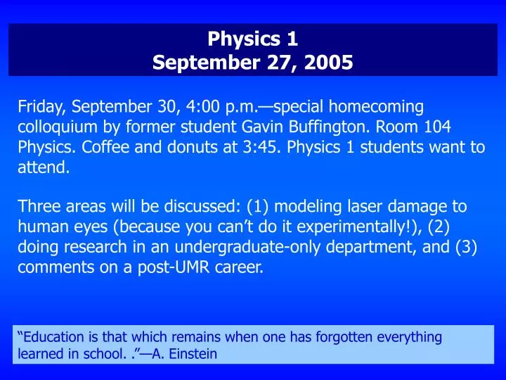
1. Physics 1 September 27, 2005 Friday, September 30, 4:00 p.m.—special homecoming colloquium by former student Gavin Buffington. Room 104 Physics. Coffee and donuts at 3:45. Physics 1 students want to attend. Three areas will be discussed: (1) modeling laser damage to human eyes (because you can’t do it experimentally!), (2) doing research in an undergraduate-only department, and (3) comments on a post-UMR career. “Education is that which remains when one has forgotten everything learned in school..”—A. Einstein

2. Chapter 6 Quantum Theory of the Hydrogen Atom 6.1 Schrödinger's Equation for the Hydrogen Atom We have discovered a "new" theory—quantum mechanics as exemplified by Schrödinger's equation. We tested it on three simple model systems in Chapter 5. We ought to test it on something a bit more “realistic,” like an atom. What’s the simplest atom you can think of? “Anyone who is not shocked by quantum theory has not understood it.”—Neils Bohr

3. The hydrogen atom is the simplest physical system containing interaction potentials (i.e., not just an isolated particle). Simple: one proton, one electron, and the electrostatic (Coulomb) potential that holds them together. The potential energy in this case is just (the attractive potential between charges of +e and –e, separated by a distance r). This is a stationary state potential (no time dependence). We could just plug it in to Schrödinger’s equation to get …but need to let the symmetry of the problem dictate our mathematical approach.

4. The spherically symmetric potential “tells” us to use spherical polar coordinates! http://hyperphysics.phy-astr.gsu.edu/hbase/sphc.html

5. Now we can re-write the 3D Schrödinger equation in three dimensions, and in spherical polar coordinates, as

6. The preceding equation can be solved for the wave function . It turns out that  is the product of three separate functions. • = Rnℓ ℓmℓmℓ , with these conditions on the quantum numbers n, ℓ, and mℓ: n= 1, 2, 3, ... ℓ= 0, 1, 2, ..., (n-1) mℓ= 0, 1, 2, 3, ..., ℓ On the next slide are the possible hydrogen electron wave functions for n=1, 2, and 3 (n=1 is the ground state).

8. Let’s look at the ground state wave function: This function contains all that is “knowable” about the ground state electron in hydrogen. The radial part is the only “interesting” part. Note that  for the ground state electron is a function of r only. You will learn in quantum mechanics that * evaluated for some state gives the probability of finding the system in that state.

9. In spherical polar coordinates, P(r)=R*Rr2dr gives the probability of finding the electron within some small dr in space centered at r. Use the 1s radial wave function and Mathcad to show that the 1s electron in hydrogen is most likely to be found at r=a0. Hints: set a0=1 for simplicity. You could use calculus to find where the radial probability function is maximum. In Mathcad it is easier to plot the probability function and see where the maximum value occurs.

10. The quantum mechanical equivalent of the average value is the expectation value, given by The expectation value of the radial part of the electron’s wave function is

11. Use Mathcad to show that the expectation value for the 1s electron’s radial coordinate is 1.5a0 (i.e., 1½ times as far from the nucleus as its most likely coordinate). Hints: set a0=1 for simplicity. Use the “integral function,” obtained by entering the “&” symbol in Mathcad. Mathcad complains if you try to integrate from 0 to . If you integrate from 0 to 50 (meaning 0a0 to 50a0 if you set a0=1), you have gone “far enough out in r” to approach infinity. Does it make sense that the average electron position is different than its most likely position? Absolutely! You may have to wait until you take Modern Physics to see why.