Abstract

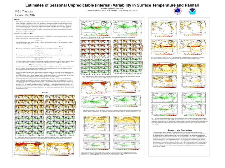
1. P-2.1 Thursday October 25, 2007 Abstract A Mean Square Error (MSE) approach is used to estimate the observed seasonal mean internal variability in rainfall and surface temperature. This method is based on the aggregation of simulations from many different Atmospheric General Circulation Models (AGCMs).A unique aspect of this particular approach is point-by-point estimation of the minimum value of mean square error (MSE) that provides an upper bound estimate for the observed seasonal mean internal (or unpredictable) variability. This methodology is implemented based on ensemble of simulations from 12 AGCMs and estimates for internal and external variance are obtained. These estimate can be updated when simulations from the next generation of models become available. Analysis procedure and data The observed seasonal mean anomalies Oj for the season “j” can be written as a sum of atmospheric response µojto SSTs and the component €ojdue to atmospheric internal variability Oj = µoj + €oj (1) The simulated ensemble mean anomaly Mjcan be written as the atmospheric response µmjand the component €mj due to atmospheric internal variability Mj = µmj + €mj (2) The estimate of observed (σ2o) and model-simulated variance of ensemble mean (σ2m) are given by σ2o = σ2oe + σ2oi (3) σ2m= σ2me + σ2mi (4) The subscripts i and e on the right hand side of Equations (3) and (4) refer to internal and external variance respectively. The Mean Square Error (MSE) of the ensemble mean prediction for a season j MSEj = (Mj - Oj)2 (5) The expected value of MSE is the sum of observed internal variability, ensemble mean of models internal variability and the error in the model simulated atmospheric response relative to the observed response to SSTs and can be written as MSE = σ2oi + σ2mi + <(µmj - µoj)2 > (6) For large ensembles and an AGCM with unbiased atmospheric response, MSE equals the observed internal variability and is the lower bound for the MSE in the paradigm of boundary-forced seasonal predictions. We use this property of MSE to estimate the internal variability of the observed seasonal means. In the present analysis, ensemble mean simulations from 11 different AGCMs are used. All the AGCM simulations are the AMIP-type long integrations and forced by the evolution of the observed SSTs. From these 11 estimates of the MSE, at each geographical location, we next find the minimum value of MSE irrespective of which AGCM it came from, and the spatial map of the minimum value of MSE is our best estimate for the observed internal variability. This method is applied to December-January-February (DJF) and June-July-August (JJA) seasonal precipitation and surface temperature data. The period of analysis for surface temperature is 1951-2000 and for precipitation is 1979-2000 respectively. The observed precipitation anomalies are from CPC CAMS-OPI and the surface temperature anomalies are from CPC CAMS analysis respectively. Model simulated precipitation and surface temperature anomalies are the ensemble mean of AGCMs. The minimum ensemble size for AGCM simulations is 7 while the maximum ensemble size is 24. We also utilize the average of ensemble mean anomalies from all 11 AGCMs and consider the average (or supersensible) as the 12 AGCM. The observed and model-simulated precipitation and surface temperature anomalies are the departure from their respective climatologies. Estimates of Seasonal Unpredictable (internal) Variability in Surface Temperature and RainfallBhaskar Jha and Arun KumarClimate Prediction Center, NCEP/NOAA, Camp Springs, MD-20746 Fig.2 variance of the observed DJF (left) and JJA (right) seasonal mean surface temperature and precipitation. The units and the Length of the period of data is same as shown in Fig.1 Fig.6. SN ratio estimate for the DJF (left) and JJA (right) seasonal mean of surface temperature and precipitation computed as the external-to-internal std dev in Fig. 5 top and Fig. 4 respectively. More ratio indicate high potential predictability. Fig.3. Mean Square Error (MSE) of the seasonal averaged DJF and JJA surface temperature and precipitation for different AGCM estimate. The units and the period of MSE computation is same shown in Fig.1. Results Fig.4 The best estimate of the internal variance of observed DJF (left) and JJA (right) surface temperature and precipitation. The best estimate is obtained from the gridpoint-by-gridpoint minimum value of MSE for different AGCMs shown in Fig.3. Fig.7. The best estimate of the internal variance (top) of observed DJF and JJA surface temperature and precipitation obtained from the coupled models (DEMETER). The estimate is the same as the one shown in Fig. 4 based on AMIP simulations. (bottom panel) the best estimate of the external variance of observed DJF and JJA surface temperature and precipitation obtained by subtracting the best estimate of the internal variance (top panel) from the total observed variance (Fig. 2). Summary and Conclusions The estimate for the internal variability of DJF and JJA observed seasonal mean surface temperature and precipitation in Fig. 4 is our best estimate of the observed internal (unpredictable) component of variability based on the current generation of AGCMs. Similarly, Fig. 7 shows the best estimate of the predictability of the seasonal atmospheric climate anomalies (surface temperature and precipitation) based on the coupled (DEMETER) data sets that include the influence of the observed ocean, atmosphere, and land initial states and as well as the influence of realistic coupling between different components of earth’s and atmosphere system. Simulations from the future generation of model integrations, and the corresponding spatial map for MSE, can be used to update the spatial map of the unpredictable component of variability in Figures 4 and 7. At the geographical locations, where the MSE for the model is higher than the current estimate, this will not lead to any update in the estimate of the unpredictable component of climate variability. These estimate can be updated when simulations from the next generation of models become available. Fig. 1. Ensemble mean variance for DJF (left) and JJA (right) seasonal mean surface temperature (degree C) and precipitation (mm./day) simulated by different AGCMs.The analysis period of surface temperature are from 1951-2000 and precipitation are from 1979-2000. Fig. 5. The best estimate of the external variance (top) of observed DJF and JJA surface temperature and precipitation obtained by subtracting the best estimate of internal variance (Fig.4) and from the observed total variance (fig.2). (bottom panel) observed surface temperature and precipitation DJF and JJA seasonal mean variance linearly related to Nino 3.4 SST.