Download
1 / 51
510 likes | 585 Views
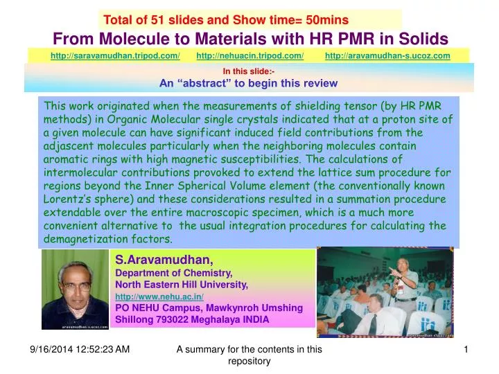
Total of 51 slides and Show time= 50mins. In this slide:- An “abstract” to begin this review. From Molecule to Materials with HR PMR in Solids. http://saravamudhan.tripod.com/ http://nehuacin.tripod.com/ http://aravamudhan-s.ucoz.com.

E N D
Total of 51 slides and Show time= 50mins In this slide:-An “abstract” to begin this review From Molecule to Materials with HR PMR in Solids http://saravamudhan.tripod.com/http://nehuacin.tripod.com/http://aravamudhan-s.ucoz.com This work originated when the measurements of shielding tensor (by HR PMR methods) in Organic Molecular single crystals indicated that at a proton site of a given molecule can have significant induced field contributions from the adjascent molecules particularly when the neighboring molecules contain aromatic rings with high magnetic susceptibilities. The calculations of intermolecular contributions provoked to extend the lattice sum procedure for regions beyond the Inner Spherical Volume element (the conventionally known Lorentz’s sphere) and these considerations resulted in a summation procedure extendable over the entire macroscopic specimen, which is a much more convenient alternative to the usual integration procedures for calculating the demagnetization factors. S.Aravamudhan, Department of Chemistry, North Eastern Hill University, http://www.nehu.ac.in/ PO NEHU Campus, Mawkynroh Umshing Shillong 793022 Meghalaya INDIA A summary for the contents in this repository
Bulk Susceptibility Effects In HR PMR SOLIDS Liquids Induced Fields at the Molecular Site Single Crystal Spherical Shape Single crystal arbitray shape Da= - 4/3 Db= 2/3 Sphere Lorentz cavity A summary for the contents in this repository
1. Experimental determination of Shielding tensors by HR PMR techniques in single crystalline solid state, require Spherically Shaped Specimen. The bulk susceptibility contributions to induced fields is zero inside spherically shaped specimen. 2. The above criterion requires that a semi micro spherical volume element is carved out around the site within the specimen and around the specified site this carved out region is a cavity which is called the Lorentz Cavity. Provided the Lorentz cavity is spherical and the outer specimen shape is also spherical, then the criterion 1 is valid. 3. In actuality the carving out of a cavity is only hypothetical and the carved out portion contains the atoms/molecules at the lattice sites in this region as well. The distinction made by this hypothetical boundary is that all the materials outside the boundary is treated as a continuum. For matters of induced field contributions the materials inside the Lorentz sphere must be considered as making discrete contributions. Illustration in next slide depicts pictorially the above sequence http://nehuacin.tripod.com/pre_euromar_compilation/index.html A summary for the contents in this repository
1. Contributions to Induced Fields at a POINT within the Magnetized Material. HighResolution Proton Magnetic Resonance Experiment Only isotropic bulk susceptibility is implied in this presentation II I SphereσII=0 Calculate σIand subtract from σexp PROTON SHIELDING σexp MolecularσM+Region IσI+Region II σII σexp= σI +σM+σII - σI = Lorentz Sphere Contribution σI≡ σinter Bulk Susceptibility Effects A summary for the contents in this repository
1. Contributions to Induced Fields at a POINT within the Magnetized Material. The Outer Continuum in the Magnetized Material Sphere of Lorentz Specified Proton Site Lorentz Sphere Lorentz Cavity The Outer Continuum in the Magnetized Material Inner Cavity surface Din Outer surface D out In the NEXT Slide: Calculation Using Magnetic Dipole Model & Equation: D out = -Din HenceD out + Din =0 The various demarcations in an Organic Molecular Single Crystalline Spherical specimen required to Calculate the Contributions to the induced Fields at the specified site. D out/in values stand for the corresponding Demagnetization Factors A summary for the contents in this repository
Equation 1 Equation 2 EUROMAR2008 If Pis related to Emac(instead of to ELoc in equation-2) which is the applied field, then the paradoxical situation would not be posed. The paradox is that ELoc is a field which is a value including the effect of P, and hence to know ELocfor equation 2 the value of P must have been known already. http://nehuacin.tripod.com/id5.html In equation 1 above ELocon the Left Hand Side of the equation, obviously depends on the value of P for estimation. And, in equation 2, the value for to is to be estimated from the value of ELoc. A summary for the contents in this repository
E3 is the discrete sum at the center of the spherical cavity; does not depend upon macroscopic specimen shape. (Lorentz field)E2is usually for only a spherical Inner Cavity; with Demagnetization factor=0.33 ; E2 = [NINNER or DINNER] x P : E1isthe contribution assuming the uniform bulk susceptibility and depend upon outer shape E1 =[NOUTER or DOUTER] x P : E0 is the externally applied field E3= intermolecular EUROMAR2008 E2= Ninnerx P http://nehuacin.tripod.com/id5.html E1=Nouterx P C.Kittel, book on Solid State Physics Pages 405-409 Lorentz Relation: Eloc = E0 +E1 + E2 +E3 A summary for the contents in this repository
Magnetic Field 6.0E-08 Each moment contributes to induced field 2 A˚ equal spacing Benzene Molecule & Its magnetic moment {χM . (1-3.COS2θ)}/(RM)3 A summary for the contents in this repository
(1-3.cos2θ) term causes +ve & -ve contributing zones See drawing below summation Lattice Shell by Shell Induced field varies as R-3 Number of molecules insuccessive shells increase as R2 Magnetic Field Product of above two vary as R-1 Each moment contributes to induced field The above distance dependences can be depicted graphically Dashed lines: convergence limit 2 A˚ equal spacing Benzene Molecule & Its magnetic moment -ve zone When the R becomes large, the R-1 term contribution becomes smaller and smaller to become insignificant {χM . (1-3.COS2θ)}/(RM)3 +ve Magnetic field direction A summary for the contents in this repository
INDUCED FIELDS,DEMAGNETIZATION,SHIELDING Induced Field inside a hypothetical Lorentz’ cavity within a specimen = H`` Shielding Factor = Demagnetization Factor = Da H`` = - . H0 = - 4 . . (Din- Dout)a . . H0 out These are Ellipsoids of Revolution and the three dimensional perspectives are imperative in = 4 . . (Din- Dout)a . When inner & outer shapes are spherical polar axis ‘a’ Din= Dout m = a/b Induced Field H`` = 0 equatorial axis ‘b’ Induced Field /4 . . . H0 = 0.333 - Dellipsoid Thus it can be seen that the the ‘D’-factor value depends only on that particular enclosing-surface shape ‘innner’ or ‘outer’ = b/a polar axis ‘b’ References to ellipsoids are as per the Known conventions-------->>>> equatorial axis ‘a’ A summary for the contents in this repository
2. Calculation of induced field with the Magnetic Dipole Model using point dipole approximations. Induced field Calculations using these equations and the magnetic dipole model have been simple enough when the summation procedures were applied as would be described in this presentation. Isotropic Susceptibility Tensor = σinter σ1 +σ2 +σ3 . . = A summary for the contents in this repository
How to ensure that all the dipoles have been considered whose contributions are signifiicant for the discrete summation ? That is, all the dipoles within the Lorentz sphere have been taken into consideration completely so that what is outside the sphere is only the continuum regime. The summed up contributions from within Lorentz sphere as a function of the radius of the sphere. The sum reaches a Limiting Value at around 50Aº. These are values reported in a M.Sc., Project (1990) submitted to N.E.H.University. T.C. stands for (shielding) Tensor Component Thus as more and more dipoles are considered for the discrete summation, The sum total value reaches a limit and converges. Beyond this, increasing the radius of the Lorentz sphere does not add to the sum significantly A summary for the contents in this repository
Within Cubic Lattice; Spherical Lorentz region ::Lattice Constant Varied 10-9.5 Eventhough the Variation of Convergence value seems widely different as it appears on Y-axis, these are within ±1.5E-08 & hence practically no field at the Centre "http://aravamudhan-s.ucoz.com/amudhan_nehu/graphpresent.html " A summary for the contents in this repository
Till now the convergence characteristics were reported for Lorentz Spheres, that is the inner semi micro volume element was always spherical, within which the discrete summations were calculated. Even if the outer macro shape of the specimen were non-spherical (ellipsoidal) it has been conventional only to consider inner Lorentz sphere while calculating shape dependent demagnetization factors. Would it be possible to Calculate such trends for summing within Lorentz Ellipsoids ? a 3rd Alpine Conference on SSNMR (Chamonix) poster contents Sept 2003. YES b Outer a/b=1 outer a/b=0.25 Demagf=0.33 Demagf=0.708 inner a/b=1 inner a/b=1 Demagf=-0.33 Demagf=-0.33 0.33-0.33=00.708-0.33=0.378 conventional combinations of shapes Fig.5[a] Conventional cases Current propositions of combinations Outer a/b=1 outer a/b=0.25 Demagf=0.33 Demagf=0.708 inner a/b=0.25 inner a/b=0.25 Demagf=-0.708 Demagf=-0.708 0.33-0.708=-0.3780.708-0.708=0 Fig.5[b] A summary for the contents in this repository
Zero Field Convergence The shape of the inner volume element was replaced with that of an Ellipsoid and a similar plot with radius was made as would be depicted Ellipticity Increases Within Cubic Lattice; Ellipsoidal Lorentz region ::Lattice Constant Varied 10-9.5 "http://aravamudhan-s.ucoz.com/amudhan_nehu/graphpresent.html " A summary for the contents in this repository
RECAPITULATION on TOPICS in SOLID STATE Defining what is Conventionally known as “Lorentz Sphere” It becomes necessary to define anInner Volume Element [I.V.E] in most of the contexts to distinguish the nearest neighbours (Discrete Region) of a specified site in solids, from the farther elements which can be clubbed in to be a continuum. The shape of the I.V.E. had always been preferentially (Lorentz) sphere. But, in the contexts to be addressed hence forth the I.V.E. need not be invariably a sphere.Even ellipsoidal I.V.E. or any general shape has to be considered and for the sake of continuity of terms used it may be referred to as Lorentz Ellipsoids / Lorentz Volume Elements. It has to be preferred to refer to hence forth as I.V.E. ( Volume element inside the solid material : small compared to macroscopic sizes and large enough compared to molecular sizes and intermolecular distances). I.V.E. need not be invariably a sphere general shape Currently:The Discrete Region Conventional Lorentz Spheres I.V.E. Shapes other than spherical For any given shape For outer shapes OR arbitrary Spherical cubical OR ellipsoidal OR A summary for the contents in this repository
2. Calculation of induced field with the Magnetic Dipole Model using point dipole approximations rs v = Volume Susceptibility r V = Volume = (4/3) rs3 2 1 v= -2.855 x 10⁻⁷ rs/r= 45.8602=‘C’ 1= 2 = 2.4 x 10⁻¹¹ for =0 A summary for the contents in this repository
"http://aravamudhan-s.ucoz.com/amudhan_nehu/3rd_Alpine_SSNMR_Aram.html" 3rd Alpine Conference On SSNMR : results from Poster A summary for the contents in this repository
Bulk Susceptibility Contribution = 0 σexp – σinter = σintra Discrete Summation Converges in Lorentz Sphere to σinter Bulk Susceptibility Contribution = 0 Similar to the spherical case. And, for the inner ellipsoid convergent σinter is the same as above σexp (ellipsoid) should be = σexp (sphere) HR PMR Results independent of shape for the above two shapes !! A summary for the contents in this repository
The questions which arise at this stage 1. How and Why the inner ellipsoidal element has the same convergent value as for a spherical inner element? 2. If the result is the same for a ellipsoidal sample and a spherical sample, can this lead to the further possibility for any other regular macroscopic shape, the HR PMR results can become shape independent ? This requires the considerations on: The Criteria for Uniform Magnetization depending on the shape regularities. If the resulting magnetization is Inhomogeneous, how to set a criterian for zero induced field at a point within on the basis of the Outer specimen shape and the comparative inner cavity shape? A summary for the contents in this repository
The reason for considering the Spherical Specimen preferably or at the most the ellipsoidal shape in the case of magnetized sample is that only for these regular spheroids, the magnetization of (the induced fields inside) the specimen are uniform. This homogeneous magnetization of the material, when the sample has uniformly the same Susceptibility value, makes it possible to evaluate the Induced field at any point within the specimen which would be the same anywhere else within the specimen.For shapes other than the two mentioned, the resulting magnetization of the specimen would not be homogeneous even if the material has uniformly the same susceptibity through out the specimen. Calculating induced fields within the specimen requires evaluation of complicated integrals, even for the regular spheroid shapes (sphere and ellipsoid) of specimen A summary for the contents in this repository
Thus if one has to proceed further to inquire into the field distributions inside regular shapes for which the magnetization is not homogeneous, then there must be simpler procedure for calculating induced fields within the specimen, at any given point within the specimen since the field varies from point to point, there would be no possibility to calculate at one representative point and use this value for all the points in the sample. A rapid and simple calculation procedure [slides # 22 to 28] could be evolved and as a testing ground, it was found to reproduce the demagnetization factor values with good accuracy which compared well with the tabulated values available in the literature. In fact, the effort towards this step wise inquiry began with the realization of the simple summation procedure for calculating demagnetization factor values. Results presented at the 2nd Alpine Conference on SSNMR, Sept. 2001 http://saravamudhan.tripod.com/ A summary for the contents in this repository
2. Calculation of induced field with the Magnetic Dipole Model using point dipole approximations. Induced field Calculations using these equations and the magnetic dipole model have been simple enough when the summation procedures were applied as described in the previous presentations and expositions. Isotropic Susceptibility Tensor = A summary for the contents in this repository
2. Calculation of induced field with the Magnetic Dipole Model using point dipole approximations For the Point Dipole Approximation to be valid practical criteria had been that the ratio r : rS= 10:1 Ri : ri = 10 : 1 or even better and the ratio Ri / ri = ‘C’can be kept constant for all the ‘n’ spheres along the line (radial vector) ‘n’ th iwill be the same for all ‘i’ , i= 1,n and the value of ‘n’ can be obtained from the equation below 1st With “C= Ri / ri , i=1,n” 3. Summation procedure for Induced Field Contribution within the specimen from the bulk of the sample. A summary for the contents in this repository
Description of a Procedure for Evaluating the Induced Field Contributions from the Bulk of the Medium Radial Vector with polar coordinates: r, θ, φ.(Details to find in 4th Alpine Conference on SSNMR presentation Sheets 6-8) http://nehuacin.tripod.com/id1.html A summary for the contents in this repository
For a given and , Rn and R1 are to be calculated and using the formula “n” along that vector can be calculated with a set constant “C” and the equation below indicates for a given and this ‘n,’ multiplied by the ‘i’ { being the same for all }would give the total cotribution from that direction = i = i=1,n,i = n, x i A summary for the contents in this repository
"http://aravamudhan-s.ucoz.com/inboxnehu_sa/nmrs2005_icmrbs.html" A summary for the contents in this repository
A spherical sample is to have a homogeneously zero induced field within the specimen. Because of the convenience with which the summation procedure can be applied to find the value of induced field not only at the center but also at any point within the specimen, it has been possible to calculate the trend for the variation of induced field from the centre to the near-surface points. There is parabolic trend observable and this seems to be the possible trend in most of the cases of inhomogeneous field distributions as well except for the values of the parabola describing this trend. It seems possible to derive parabolic parameter values depending on the shape factors in the case of inhomogeneous field distributions in the non-ellipsoidal shapes. This would greatly reduce the necessity to do the summing over all the θ and φ values. This possiblility has been illustrate (in anticipation of the verification of the trends) in the remaining presentation in particular the last four slides. A summary for the contents in this repository
Using the Summation Procedure induced fields within specimen of TOP (Spindle) shape and Cylindrical shape could be calculated at various points and the trends of the inhomogeneous distribution of induced fields could be ascertained. Poster Contribution at the 17thEENC/32ndAmpere, Lille, France, Sept. 2004 Graphical plot of the Results of Such Calculation would be on display Zero ind. Field Points A summary for the contents in this repository
The top or a Spindle Shaped object comes under the category of Shapes within which the Induced field distribution would be Inhomogeneous even if the Susceptibility is uniformly the same over the entire sample NMR Line for only Intra molecular Shielding Added intermolecular Contribultions causes a shiftdownfieldorupfield homogeneous Inhomogeneous Magnetization can Cause Line shape alterations 4. The case of Shape dependence for homogeneously magnetized sample, and consideration of in-homogeneously magnetized material. A summary for the contents in this repository
The induced field distribution in materials which inherently possess large internal magnetic fields, or in materials which get magnetized when placed in large external Magnetic Fields, is of importanceto material scientists to adequately categorize the material for its possible uses. It addresses to the questions pertaining to the structure of the material in the given state of matter by inquiring into the details of the mechanisms by which the materials acquire the property of magnetism. To arrive at the required structural information ultimately, the beginning is made by studying the distribution of the magnetic field distributions within the material (essentially magnetization characteristics) so that the field distribution in the neighborhood of the magnetized (magnetic) material becomes tractable. The consequences external to the material due the internal magnetization is the prime concern in finding the utilization priorities for that material. In the materials known conventionally as the magnetic materials, the internal fields are of large magnitude. To know the magnetic field inducing mechanisms to a greater detail it may be advantageous to study the trends and patterns with a more sensitive situation of the smaller variations in the already small values of induced fields can be studied and the Nuclear Magnetic Resonance Technique turns out to be a technique, which seems suitable for such studies. When the magnetization is homogeneous through out the specimen, it is a simple matter to associate a demagnetization factor for that specimen with a given shape-determining factor. When the magnetized (magnetic) material is in-homogeneously magnetized, then a single demagnetization factor for the entire specimen would not be attributable but only point wise values. Then can an average demagnetization factor be of any avail and how can such average demagnetization factor be defined and calculated .It is a tedious task to evaluate the demagnetization factor for homogeneously magnetized, spherical (ellipsoidal) shapes. An alternative convenient mathematical procedure could be evolved which reproduces the already available tables of values with good accuracy. With this method the questions pertaining to induced field calculations and the inferences become more relevant because of the feasibility of approaches to find answers. A summary for the contents in this repository
Correlating ‘r’ and ‘r -3’ Calculation of the Induced Field Distribution in the region outside the magnetized spherical specimen A summary for the contents in this repository
http://aravamudhan-s.ucoz.com/amudhan20012000/ismar_ca98.htmlhttp://aravamudhan-s.ucoz.com/amudhan20012000/ismar_ca98.html A summary for the contents in this repository
Advantages of the summation method described in the previous sheets: (An alternative method for demagnetization factor calculation): Also at http://www.geocities.com/inboxnehu_sa/nmrs2005_icmrbs.html 1. First and Foremost, it was a very simple effort to reproduce the demagnetization factor values, which were obtained and tabulated in very early works on magnetic materials. Those Calculations which could yield such Tables of demagnetization factor values were rather complicated and required setting up elliptic integrals which had to be evaluated. 2. Secondly, the principle involved is simply the convenient point dipole approximation of the magnetic dipole. And, the method requires hypothetically dividing the sample to be consisting of closely spaced spheres and the radii of these magnetized spheres are made to hold a convenient fixed ratio with their respective distances from the specified site at which point the induced fields are calculated. This fixed ratio is chosen such that for all the spheres the point dipole approximation would be valid while calculating the magnetic dipole field distribution. 3. The demagnetization factors have been tabulated only for such shapes and shape factors for which the magnetization of the sample in the external magnetic field is uniform when the magnetic susceptibility of the material is the same homogeneously through out the sample. This restricts the tabulation to only to the shapes, which are ellipsoids of rotation. Where as, if the magnetization is not homogeneous through out the sample, then, there were no such methods possible for getting the induced field values at a point or the field distribution pattern over the entire specimen. The present method provides a greatly simplified approach to obtain such distributions. 4. It seems it is also a simple matter, because of the present method, to calculate the contributions at a given site only from a part of the sample and account for this portion as an independent part from the remaining part without having to physically cause any such demarcations. This also makes it possible to calculate the field contribution from one part of the sample, which is within itself a part with homogeneously, magnetized part and the remaining part being another homogeneously magnetized part with different magnetization values. Hence a single specimen which is inherently in two distinguishable part can each be considered independently and their independent contribution can be added. For the point 1 mentioned above view Calculation of Induced Fileds Outside the specimen http://nehuacin.tripod.com/id3.html http://saravamudhan.tripod.com/ A summary for the contents in this repository
The task would be to calculate the induced field inside the cavity σcavity Organic Molecular single crystal : a specimen of arbitrary shape Induced field calculation by discrete summation σinter I.V.E Sphere Continuum σIVE = σinter + σM Discrete I.V.E. Cavity Added σinter Shifts the line position O σcavity = σBulk +σM InnerVolume Element I.V.E H O MRSFall2006 σintra / σM O O 4 point star indicates the molecule at a central location. Structure of a typical molecule on the right σIVE(S) σM O H In-homogeneity can cause line shape alterations: O Proton Site with σintra not simply shifts only single sharp line A summary for the contents in this repository
A cylinder shaped specimen (Blue line in the plot below) The points on the Blue line would be specified and at these Calculated field values an NMR line would be placed after adding the sum total of intra and intermolecular contributions to induced fields. Calculations at 9 points along the axis Zero ind. Field Points Not to be discussed in this presentation Distance along the axis MRSFall2006 http://nehuacin.tripod.com/id1.html A summary for the contents in this repository
Add to all Values down the column “Only”inter-molecular value5.80E-07 was added and the line shape was plotted with those values : NEXT GRAPHICAL PLOT A Graph of the data in table Overlapping last three lines Lines at interpolated values Onlyinter molecular value5.80E-07 can be set = 0 No intra molecular Value; inter- molecular value (in I.V.E) set=0 in subsequent plots; only cavity field is used to generate line shapes A summary for the contents in this repository
Same graph as displayed in previous slide Gradual increase of component lines broadens the lines and can cause the change in the appearance of overall shape. Illustration with4 different width values 10 times that of red Width 2.5 times that of green Width twice that of blue Width twice that of red Same width as above A summary for the contents in this repository
Line at σIVE A summary for the contents in this repository
1.Reason for the conevergence value of the Lorentz sphere and ellipsoids being the same. Added Results to be discussed at 4th Alpine Conference http://nehuacin.tripod.com/id3.html 2.Calculation of induced fields within magnetized specimen of regular shapes. (includes other-than sphere and ellipsoid cases as well) 3. Induced field calculations indicate that the point within the specimen should be specified with relative coordinate values. The independent of the actual macroscopic measurements, the specified point has the same induced field value provided for that shape the point is located relative to the standardized dimension of the specimen. Which means it is only the ratios are important and not the actual magnitudes of distances. Further illustrations in next slide The two coinciding points of macroscopic specimen and the cavity are in the respective same relative coordinates. Hence the net induced field at this point can be zero These two points would have the same induced field values (both at ¼) These two points would have the same induced field values (both midpoints) Lorentz cavity A summary for the contents in this repository
Symbols for Located points Applying the criterion of equal magnitude demagnetization factor and opposite sign Inside the cavity Points in the macroscopic specimen This type of situation as depicted in these figures for the location of site within the cavity at an off-symmetry position, raises certain questions for the discrete summation and the sum values. This is considered in the next slide ⅛ specimen length ⅛ cavity length In the cavity the cavity point is relatively at the midpoint of cavity. The point in bulk specimen is relatively at the relative ¼ length. Hence the induced field contributions cannot be equal and of opposite sign Relative coordinate of the cavity point and the Bulk specimen point are the same. Hence net induced field can be zero A summary for the contents in this repository
For a spherical and ellipsoidal inner cavity, the induced field calculations were carried out at a point which is a center of the cavity . In all the above inner cavities, the field was calculated at a point which is centrally placed in the inner cavity. Hence the discrete summation could be carried out about this point of symmetry. This is the aspect which will have to be investigated from this juncture onwards after the presentation at the 4th Alpine Conference. The case of anisotropic bulk susceptibility can be figured out without doing much calculations further afterwards. If the point is not the point of symmetry, then around this off-symmetry position the discrete summation has to be calculated. The consequence of such discrete summation may not be the same as what was reported in 3rd Alpine conference for ellipsoidal cavities, but centrally placed points. A summary for the contents in this repository
This stage of the Report was possible because of the beginning made as early as 1979-80 to be concerned with the Induced field distributions inside the specimen in connection with the HR PMR in Single Crystal solids. A careful consideration of the demagnetization Calculations the results of which had been reported in the form of documented tables revealed that a pattern can be setup with a simplified form but the question was how to translate this criteria in the form of a concrete mathematical equations. An intense effort (which could have elicited a comment as a futile effort from active researchers in the related area) did result in a form for the equation, the derivation of which turned out to be requiring only four to five elementary steps. Equipped with this formulation and equation in hand it did not take any more than half an hour to one hour to arrive at the Zero Induced field value at the centre of the Lorentz Cavity in a spherically shaped magnetized specimen. Then it was a question of arriving at the reported numerical values for the ellipsoids of different shape-factor ratios the 'm' and the 'µ' (reciprocal of 'm') . It took about one month to incorporate the ellipsoidal equation criteria and get a few reported demagnetization factors. All this could be achieved by simple hand calculations - not even a pocket calculator to use. http://nehuacin.tripod.com/pre_euromar_compilation/id5.html This was the result in hand as early as 1984. Afterwards,since there were not many who would have wanted to know about these ( because the demagnetization factors were already available in Tables since long before), the results were stored as they were in a scribbling pad filled with numbers due to the hand calculations. By that time all the references which have been gathered (these are all listed out in the website http://saravamudhan.tripod.com, in the page for the '2nd Alpine conference on SSNMR'; CLICK on this pane to display the webpage)indicated that a reference(# 17) in the Physical review publication from authors from Washington, St Louis Missourie,USA had some what similar effort reported. A summary for the contents in this repository
What was referred to before is a publication by an Indian author who worked and submitted a dissertation at E.T.H., Zurich, Switzerland. This work had been also published in Pure and Applied Geophysics. I had tried to get the referred issue from the Geophysical Research Institute at Hyderabad and I mentioned about this to Dr.A.C.Kunwar at IICT, Hyderabad, as early as 1995-96. By that time I had been at the North Eastern Hill University, shillong as Lecturer in Chemistry and as excercises to M.Sc., students I had suggested these simple equations and susceptibility induced fields in magnetized specimen to work for their 6-months project report successively for about 4-5 years. This resulted in a computer program to calculate these induced field contributions and 6 project reports consisted of consecutive materials. There was not much interest from any to these equations and results, presumably, even at that time in my opinion which could be because all the demagnetization factors are well reported and, whether now it is simplified calculation or not,it is merely a question of simplification but the possible values were already well documented.After about two years in 1998 I received by POST the reprint of the publication by P.V.Sharma (in Geophysical Research journal) from Dr.A.C. Kunwar. This paper contained a rapid computation method for such calculations and my considerations were even simpler. And hence from the NMRS symposium at Dehradun in 1999, I have been presenting my consideration by way of Poster/oral presentations and the support I had for presenting them has resulted in this kind of a activity requiring them to be reported in International Conferences. During the period till now these efforts had encouragements from the NMRS, ISMAR and the Congress Ampere and occasional finacial support from these organizers and the Funding agencies CSIR, INSA have gone a long way in pusrsuing the efforts with the possible provisions at the North Eastern Hills University, which is gratefully acknowledged A summary for the contents in this repository
IBS Meeting : Symposium at BHU, 2010 Prof. S. Aravamudhan, receiving a memento after Chairing a technical session From Prof. P.C.Mishra Convener, IBS 2010 A summary for the contents in this repository
International Biophysics ConferenceIUPAB. At Buenos Aires, Argentina April-May 2002 S.Aravamudhan and K.Akasaka IBS Meeting 2002, CBMR, SGPGIMS, Lucknow Amitabha Chattopadhyaya NR Krishana A generous grant from the WELCOME TRUST UK enabled the participation of Dr.S.Aravamudhan in the International Biophysics Conference at Buenos Aires, Argentina which is gratefully acknowledged. A summary for the contents in this repository