Download
1 / 65
650 likes | 658 Views
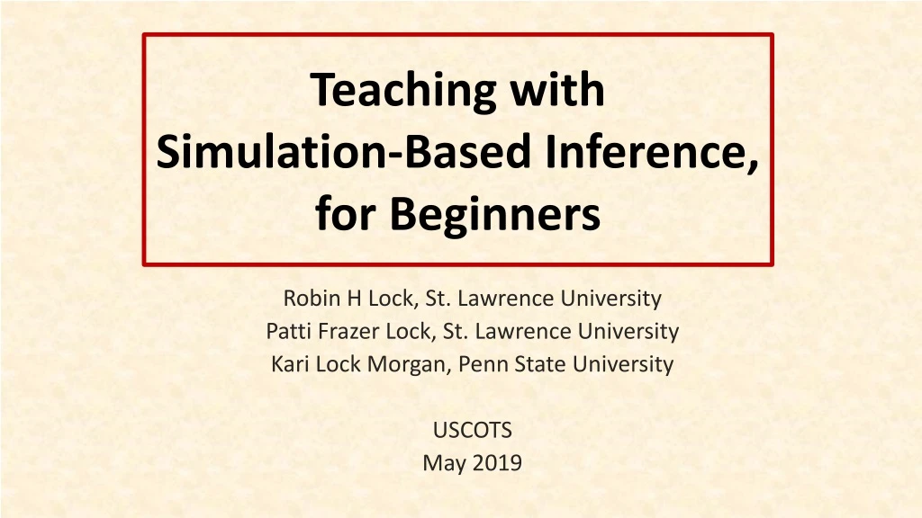
Teaching with Simulation-Based Inference, for Beginners. Robin H Lock, St. Lawrence University Patti Frazer Lock, St. Lawrence University Kari Lock Morgan, Penn State University USCOTS May 2019. The Lock 5 Team. Kari [Harvard] Penn State. Eric [North Carolina] Minnesota. Dennis

E N D
Teaching with Simulation-Based Inference, for Beginners Robin H Lock, St. Lawrence University Patti Frazer Lock, St. Lawrence University Kari Lock Morgan, Penn State University USCOTS May 2019
The Lock5 Team Kari [Harvard] Penn State Eric [North Carolina] Minnesota Dennis [Iowa State] Buffalo Bills Patti & Robin St. Lawrence
Introductions: Name Institution Experience
GOAL • Use • Simulation Methods • to • increase understanding • reduce prerequisites • Increase student success
How much variation is there in the sample statistics if n = 56? Example: We wish to estimate p = the proportion of Reese’s Pieces that are orange. Find the proportion in your sample. (Then feel free to eat the evidence!)
How much variation is there in the sample statistics if n = 56? We get a better sense of the variation if: We have thousands of samples!
We need technology!! StatKey!! www.lock5stat.com/statkey Free, online, works on all platforms, easy to use
Created from the population • Centered at the population parameter • Bell-shaped • Shows variability in sample statistics (Standard Error = standard deviation of sample statistics given a fixed sample size) Sampling Distribution
In order to create a sampling distribution, we need to already know the population parameter or be able to take thousands of samples! Sampling Distribution: Big Problem!! Not helpful in real life!!
Key Concept: Variability in Sample Statistics • Overview for Today: • Two simulated distributions for a statistic • Emphasize the key concept of variability • Are extremely useful in doing statistics
Simulated Distribution #1 • Created using only the sample data • Centered at the sample statistic • Bell-shaped • Same Variability/Standard Error !!! Bootstrap Distribution (for Confidence Intervals)
Simulated Distribution #2 • Created assuming a null hypothesis is true • Centered at the null hypothesis value • Bell-shaped • Same Variability/Standard Error !!! (assuming the null hypothesis is true) Randomization Distribution (for Hypothesis Tests)
Key Concept: Variability in Sample Statistics • Sampling Distribution • Created from the population • Centered at population parameter • Bell-shaped • Gives variability/standard error • Simulated Distribution #1 • Created from the sample • Centered at sample statistic • Bell-shaped • Gives variability/standard error • Simulated Distribution #2 • Created assuming null is true • Centered at null value • Bell-shaped • Gives variability/standard error
This material can come very early in a course. It requires only basic knowledge of summary statistics and sampling. Let’s get started…
Bootstrap Confidence Intervals How can we estimate the variability of a statistic when we only have one sample?
Assessing Uncertainty • Key idea: how much do statistics vary from sample to sample? • Problem? • We can’t take lots of samples from the population! • Solution? • (re)sample from our best guess at the population – the sample itself!
Original Sample A simulated “population” to sample from
Bootstrap Sample: Sample with replacement from the original sample, using the same sample size. Original Sample Bootstrap Sample
BootstrapSample Bootstrap Statistic BootstrapSample Bootstrap Statistic Original Sample Bootstrap Distribution • ● • ● • ● ● ● ● Sample Statistic BootstrapSample Bootstrap Statistic
Example: Mustang Prices Start with a random sample of 25 prices (in $1,000’s) Goal: Find an interval that is likely to contain the mean price for all Mustangs Key concept: How much can we expect means for samples of size 25 to vary just by random chance?
Original Sample Bootstrap Sample Repeat 1,000’s of times!
We need technology!! StatKey!! www.lock5stat.com/statkey
How do we get a CI from the bootstrap distribution? • Method #1: Standard Error • Find the standard error (SE) as the standard deviation of the bootstrap statistics • Find an interval with
Sample Statistic Standard Error )
How do we get a CI from the bootstrap distribution? • Method #1: Standard Error • Find the standard error (SE) as the standard deviation of the bootstrap statistics • Find an interval with • Method #2: Percentile Interval • For a 95% interval, find the endpoints that cut off 2.5% of the bootstrap means from each tail, leaving 95% in the middle
95% CI via Percentiles Keep 95% in middle Chop 2.5% in each tail Chop 2.5% in each tail We are 95% sure that the mean price for Mustangs is between $11,918 and $20,290
99% CI via Percentiles Keep 99% in middle Chop 0.5% in each tail Chop 0.5% in each tail We are 99% sure that the mean price for Mustangs is between $10,878 and $21,502
Bootstrap Confidence Intervals Version 1 (Statistic 2 SE): Great preparation for moving to traditional methods Version 2 (Percentiles): Great at building understanding of confidence level
Bootstrap Approach • Create a bootstrap distribution by simulating many samples from the original data, with replacement, and calculating the sample statistic for each new sample. • Estimate confidence interval using either statistic ± 2 SE or the middle 95% of the bootstrap distribution. Same process works for different parameters!
Your Turn! Three more examples.
Example #1: Atlanta Commutes What’s the mean commute time for workers in metropolitan Atlanta? Data: The American Housing Survey (AHS) collected data from Atlanta. We have a microdata sample of 500 commuters from that sample. Find a 95% confidence interval for the mean commute time for all Atlanta commuters.
Example #2: News Sources How do people like to get their news? A recent Pew Research poll asked “ Do you prefer to get your news by watching it, reading it, or listening to it?” They found that 1,164 of the 3,425 US adults sampled said they preferred reading the news. Use this information to find a 90% confidence interval for the proportion of all US adults who prefer to get news by reading it. https://www.journalism.org/2018/12/03/americans-still-prefer-watching-to-reading-the-news-and-mostly-still-through-television/
Example #3: Diet Cola and Calcium How much does diet cola affect calcium excretion? In an experiment, 16 healthy women were randomly assigned to drink 24 ounces of either diet cola or water. Calcium loss (in mg) was measured in urine over the next few hours. Use this information to find a 95% confidence interval for the difference in mean calcium loss between diet cola and water drinkers. Larson, N.S. et al, ‘Effect of Diet Cola on Urine Calcium Excretion”, Endocrine Reviews, 2010.
Sampling Distribution Population BUT, in practice we don’t see the “tree” or all of the “seeds” – we only have ONE seed µ
Using only the Sample Data What can we do with just one seed? “Simulated Population” Estimate the distribution and variability (SE) of ’s from this new distribution Grow a NEW tree! µ
Randomization Hypothesis Tests Key Concept: How do we measure strength of evidence?
Example: Beer & Mosquitoes Question: Does consuming beer attract mosquitoes? Experiment: 25 volunteers drank a liter of beer, 18 volunteers drank a liter of water Randomly assigned! Mosquitoes were caught in traps as they approached the volunteers.1 1Lefvre, T., et. al., “Beer Consumption Increases Human Attractiveness to Malaria Mosquitoes, ” PLoS ONE, 2010; 5(3): e9546.
Beer and Mosquitoes Number of Mosquitoes Beer 27 20 21 26 27 31 24 19 23 24 28 19 24 29 20 17 31 20 25 28 21 27 21 18 20 Water 21 22 15 12 21 16 19 15 24 19 23 13 22 20 24 18 20 22 Beer mean = 23.6 Water mean = 19.22 Beer mean – Water mean = 4.38 Does drinking beer actually attract mosquitoes or is the difference just due to random chance?
Beer and Mosquitoes Number of Mosquitoes What kinds of results would we see, just by random chance, if there were no difference between beer and water? Beer 27 20 21 26 27 31 24 19 23 24 28 19 24 29 20 17 31 20 25 28 21 27 21 18 20 Water 21 22 15 12 21 16 19 15 24 19 23 13 22 20 24 18 20 22
Beer and Mosquitoes Number of Mosquitoes What kinds of results would we see, just by random chance, if there were no difference between beer and water? Beer 27 20 21 26 27 31 24 19 23 24 28 19 24 29 20 17 31 20 25 28 21 27 21 18 20 Water 21 22 15 12 21 16 19 15 24 19 23 13 22 20 24 18 20 22 27 19 21 24 20 24 18 19 21 29 20 23 26 20 21 13 27 27 22 22 31 31 15 20 24 20 12 24 19 25 21 18 23 28 16 20 24 21 19 22 28 27 15 We can find out!! Just re-randomize the 43 values into one pile of 25 and one of 18, simulating the original random assignment.
Beer and Mosquitoes Number of Mosquitoes What kinds of results would we see, just by random chance, if there were no difference between beer and water? Beer Water 24 20 24 18 19 21 29 20 23 26 20 21 13 27 27 22 22 31 31 15 20 24 20 12 24 19 25 21 18 23 28 16 20 24 21 19 22 28 27 15 27 19 21 20 24 19 20 24 31 13 18 24 25 21 18 15 21 16 28 22 19 27 20 23 22 21 20 26 31 19 23 15 22 12 24 29 20 27 21 17 24 28 Compute the beer mean minus water mean of this simulated sample. Do this thousands of times!
We need technology!! StatKey!! www.lock5stat.com/statkey
P-value This is what we saw in the experiment. This is what we are likely to see just by random chance if beer/water doesn’t matter.
Beer and Mosquitoes • The Conclusion! The results seen in the experiment are very unlikely to happen just by random chance (less than 1 out of 1000!) We have strong evidence that drinking beer does attract mosquitoes!
What about the traditional approach? “Students’ approach to p-values … was procedural … and [they] did not attach much meaning to p-values” -- Aquilonius and Brenner, “Students’ Reasoning about P-Values”, SERJ, November 2015
Another Look at Beer/Mosquitoes 1. Check conditions 2. Which formula? 5. Which theoretical distribution? 6. df? 7. Find p-value 8. Interpret a decision 3. Calculate numbers and plug into formula 4. Chug with calculator 0.0005 < p-value < 0.001
P-value This is what we saw in the study. This is what we are likely to see just by random variation if the null hypothesis is true.