Department of Earth Science and Engineering Imperial College London Meng-Che Wu

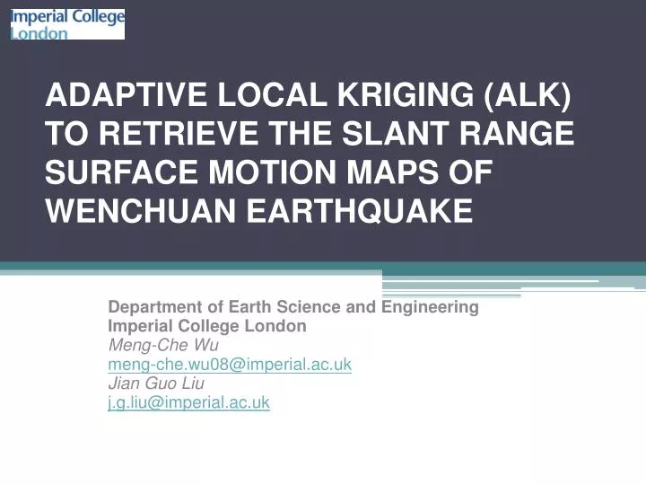
ADAPTIVE LOCAL KRIGING (ALK) TO RETRIEVE THE SLANT RANGE SURFACE MOTION MAPS OF WENCHUAN EARTHQUAKE Department of Earth Science and Engineering Imperial College London Meng-Che Wu meng-che.wu08@imperial.ac.uk JianGuo Liu j.g.liu@imperial.ac.uk

Outline • Background & Purpose • Method Development • Experimental Results • Conclusions • Future works

Background & Purpose

Path 471 Path 472 Background & Purpose Path 474 Path 475 Path 476 2π Path 473 Azimuth Range 0

Path 471 Path 472 Background & Purpose Path 474 Path 475 Path 476 ≈ 1 m Path 473 Azimuth Range ≈ -1 m

Ordinary kriging concept Ordinary kriging: Γ * λ = g Γ is a matrix of the semivariance between each sampled point. λ is a vector of the kriging weights. g is a vector of the semivariancebetween a unknown point and each sampled point. Semivariance = FSM(D) FSM is the fitted semivariogram model. D is the distance bewteen each sampled point or the distance between a unknown point and each sampled point. S = (x, y) is a location

Example of semivariogram model Gaussian model ≈ 1 m ≈ -1 m

Method: Adaptive Local Kriging Hang wall Window based krigingscan to calculate the linear fitting of local semivariance. 2. Window size is locally adaptive to ensure adequate data points and high processing efficiency. ≈ 1 m Azimuth Range Foot wall ≈ -1 m

ALK local semivariogram model: Towards the seismic fault (Hang wall side) Local gradient: 1.258×10-5 Semivariance Distance Averaged semivariance Fitted semivariance x = 1024, y = 230

ALK local semivariogram model: Towards the seismic fault (Foot wall side) Local gradient: 1.624×10-5 Semivariance Distance Averaged semivariance Fitted semivariance x = 745, y = 1200

Give some sampled points in the large decoherence gaps H Ordinary kriging ALK multi-step processing flow chart F Coherence thresholding Final ALK result Input data Hang wall & foot wall separation Coherence thresholding ALK (Decoherence zone) H ALK Artificial discontinuity elimination F

ALK data ≈ 1 m Azimuth Range ≈ -1 m

ALK rewrapped interferogram 2π Azimuth Range 0

Original interferogram 2π Azimuth Range 0

Path 471 profiles ALK results assessment A A A’ RMSE: 0.0053591572 meters Correlation coefficient: 0.99999985 Original unwrapped image profile A’ Azimuth ALK data profile Range ≈ 1 m ≈ -1 m

Path 472 profiles ALK results assessment A A A’ RMSE: 0.00909682429 meters Correlation coefficient: 0.99939712 Original unwrapped image profile Azimuth A’ ALK data profile Range ≈ 1 m ≈ -1 m

Path 473 profiles ALK results assessment A A’ A RMSE: 0.0083477924 meters Correlation coefficient: 0.99973365 Original unwrapped image profile Traced fault line Initial fault Azimuth A’ ALK data profile Range ≈ 1 m ≈ -1 m

Path 476 profiles ALK results assessment A A’ A RMSE: 0.0071013203 meters Correlation coefficient: 0.99929831 Original unwrapped image profile Azimuth A’ ALK data profile Range ≈ 1 m ≈ -1 m

3D visualization of ALK data ≈ 1 m ≈ -1 m

Refined ALK data ≈ 1 m Azimuth Range ≈ -1 m

Refined ALK rewrapped data 2π Azimuth Range 0

3D view of refined ALK unwrapped data ≈ 1 m ≈ -1 m

Conclusions • Local semivariogramis more representive to the local variation of spatial pattern of the interferogram than a global semivariogram model. • Dynamical local linear model represents a nonlinear global model for the whole interferogram. • ALK multi-step processing procedure avoids the error increases in large decoherence gaps.

Conclusions • The ALK interpolation data revealed dense fringe patterns in the decoherencezone and show high fidelity to the original data without obvious smoothing effects. • The initial fault line separating the data does not affect the final interpolation result of ALK processing. • The seismic fault line that can be denoted in the ALK is different from that in publications. The discrepancy needs further investigation.

Future works • Geological structural numerical modeling to explain the discrepancy of trend of seismic fault line. • Three dimensional surface deformation maps development.

Thank you Any questions ?

Department of Earth Science and Engineering Imperial College London Meng-Che Wu