Download
1 / 41
420 likes | 429 Views
Ophthalmic Doctorate Advanced Visual Science Crowding and Summation TSM3. Dr Tim S. Meese t.s.meese@aston.ac.uk. Last updated: Sept 16 th 2010. Key References.

E N D
Ophthalmic DoctorateAdvanced Visual ScienceCrowding and SummationTSM3 Dr Tim S. Meese t.s.meese@aston.ac.uk Last updated: Sept 16th 2010
Key References The references in this list either (1) make an important contribution to the points developed in this lecture or (2) provide valuable reviews or expositions; or both. All are recommended reading. Highlights indicate essential reading You will be directed to these at appropriate junctures during the PPT. You will also be given a few exercises to perform highlighted in red. The PPT might also include other references not included in this list which are less central to understanding the lecture. • CROWDING • Levi (2008) • Martelli, Majaj & Pelli (2005) • Parkes, Lund, Angelucci, Solomon & Morgan (2001) • Pelli & Tillman (2008) • Petrov, Popple & McKee (2007) • There is a special issue on crowding in the ‘on-line’ Journal of Vision, 2008 volume 7, No 2. Well worth a browse. • CONTRAST SUMMATION • Meese & Summers (2007) • Meese & Williams (2000) • Meese (2010) • Robson & Graham (1981)
Prologue • In this lecture we focus on two issues that have tended to be treated separately in the literature: crowding (Part 1) and spatial summation of contrast (Part 2). • The two parts of this lecture can be treated independently (e.g. like two lectures), but there are tantalizing hints that they might be more closely related than previously thought. • Much of the content of Part 1 is influenced by two recent reviews of the subject by Pelli & Tillman (2008) and Levi (2008). • The presentation of the material in Part 1 is quite ‘light’, whereas Part 2 is more technically demanding.
PART 1 • Crowding
Where’s the butter? There are two factors here. The first is that you had to search a cluttered scene to find a target item. This process is known as visual search and it has been researched extensively. This is not the focus of this lecture. • Click to find out The second is that the representation of objects away from the fovea is not very good. Perhaps this is not surprising, after all we now that spatial resolution is poor in the periphery. But look directly at the ‘thank you’ bag and then click to remove everything except the butter. You can detect the butter with this peripheral part of your retina. It’s just that before, it was being hidden from awareness by all the surrounding objects. This phenomenon is known as crowding, and it means that it is difficult for targets to attract your attention when embedded in cluttered scenes. To convince yourself of this point, try going back to the beginning of this slide sequence, fixate the ‘thank you’ bag and attend to the butter. The butter tends to come and go form visual awareness.
Why is crowding interesting? • Object recognition (e.g. knowing a car is a car) is one of the main goals of visual perception. • But it is not very well understood! • Crowding interferes with recognition and so one line of thought is that if we can understand what’s happening to cause crowding then we are one step closer to understanding object recognition. • It is relevant to reading. • It is probably important for several clinical conditions including: • Dyslexia • Macular degeneration • Amblyopia • Some forms of agnosia
Typical experimental demonstration of crowding • Vision scientists rarely do experiments with fridges and butter, but text and letters are also meaningful real world objects and are much easier to manipulate in the laboratory. • First fixate the red spot then click to introduce a letter and try and identify it. • That was easy, but now click and try again. • It is now much harder (impossible?) to recognize the R because of crowding from the other letters: the target and the flankers all jumble together and become confused. K R E A Z
Some basic experimental findings • As we have seen, crowding is not simply due to a loss of acuity in the periphery, because unflanked targets can be correctly identified. • Crowding has been found for many classes of stimuli, not just letters (e.g. see Journal of Vision special issue). • Crowding is either very weak or absent in the fovea (see Levi, 2008). • Crowding is not isotropic (Toet & Levi, 1992): for the configuration below, experiments confirm that the effect of horizontally placed flanks is greater than vertically placed flanks … C H C P P H
Some basic experimental findings • …but the situation is reversed for the configuration shown on this slide. • In other words, crowding is most severe along contours that radiate out from the fovea. H C P C P H
The Bouma Law and critical spacing • The ‘critical spacing’ is often treated as the smallest distance between the target and the nearest flanker that is needed for the target to be reliably identified. Often this measure is taken as the distance between the centres of the objects (letters). • Experiments have shown that • The critical spacing does not depend on object size (this was quite surprising because it had long been believed that acuity was the important factor). • Based on (often overlooked) observations made by Bouma in the 1970s, and not forgetting the importance of direction from target to flankers (previous slides), Pelli & Tillman (2008) describe the Bouma Law thus: the critical spacing of crowding depends solely on location and direction. Broadly speaking, the critical spacing is about 50% of the eccentricity. • However, although critical spacing does not depend on objects it does depend on individuals. That is, different people have different critical spacing. • In fact, it turns out that there is a further complicating factor, which is that for some people there is a quadratic component to the critical spacing. This is to say that the critical spacing, s = s1 + s2e + s32e, where e is eccentricity and s1,s2 ands3 are specific to different people. This modification to the Bouma Law provides a good account of a wide body of data(Pelli, Tillman, Freeman et al, 2007).
Critical spacing and cortical magnification • The Bouma Law makes sense in terms of what is known about the cortical magnification factor (mm of cortex per deg of visual angle). • The magnification factor scales with eccentricity • 1 mm diameter patches of retina project to smaller contiguous regions of primary visual cortex the further you move away from the fovea. • Thus, the cortex magnifies the foveal representation of the image relative to the periphery. • The result of cortical magnification is that critical spacing maps to a constant cortical space for all eccentricities. According to Pelli & Tillman (2008), typical critical spacing corresponds with about 6mm of cortex.
Crowding is characterized by two parameters • Parameter 1. The critical spacing of crowding (see previous slide). • Parameter 2. The amplitude of crowding. This measure depends on the stimulus. For example, in experiments using aligned Gabor patches, the magnitude of crowding might be the level of orientation difference between target and flankers. In experiments using letters it might be the contrast of the letter needed to identify it. • In sum: parameter 1 describes the radius of influence of crowding and parameter 2 describes the magnitude of the effect. • According to Pelli & Tillman (2008) the value of parameter 1 is fairly constant, but the value of parameter 2 can depend on stimulus type.
The uncrowded window • Because the critical distance is so small in the fovea, there is an uncrowded window through which we view the world. (This is sometimes called the uncrowded span.) • Below is an example adapted from Pelli, Tillman, Freeman et al (2007). Look directly at the red spot. • The central region of text looks fine, and it is fine. The surrounding text is jumbled, but when we look centrally we don’t notice because the normal operation of crowding means that we expect text and objects to appear jumbled in that large region anyway! In other words, whether the text is jumbled or not on the page, it becomes jumbled by the visual system and we can’t read it. Rof mreo nath 25 eayrs, distues fo spalati ivison vhae enbe midoednat yb het eiwv hatt tispaal racstont olinpog si akwe ta ctiondete hretshdol (g.e. probability sumatomin). Htsi eivw aws fsirt halclendge ni our recent companion parpe (Eseme & Merssum, 2007), where we concluded thta a gnsial mbconatioin sttraeyg aktes lapce across several grating cyclse ta thersohdl nad aobev. In hte binocular domain, Seeme te la (0026) cerentyl onccledud ttah ncotrast summation arocss esye si gterrea thna teh orfact fo 2√ (d3B, ro uaqdrcait smutmaoin) tath sah otfne eben sseduppo (Amcpblle & Reegn, 6159).
Implications for reading • The crowding effects of text don’t usually cause a problem for normal readers because we make rapid eye-movements (about 4 per second) so that the text that we are attending is always placed within the uncrowded window. • If text is made smaller it is more difficult to read. In the past this was attributed to acuity. However, when text is made smaller, it is usually packed more closely and this causes crowding. Thus, very small text can be made easier to read by increasing the space between the letters and words. Stand back a few feet and try reading the blue text that appears on the next click. (The font size is the same for the bottom two lines) • However, the issue turns out to be quite complex. The interested reader is referred to Pelli, Tillman, Freeman et al (2007) and Levi, Song & Pelli (2007). Big text is easy to read Small text is much more difficult to read B u t i s e a s i e r w h e n s p a c e s a r e i n s e r t e d
Face perception • Instructions: Hold fixation on the red spot and then click to make a face appear. See if you can recognize this famous face without moving your eyes. Then shift your gaze to the face to check. • Now do it.
Face perception • The difficulty in recognizing faces in the periphery has often been attributed to poor visual resolution. • However, Martelli et al (2005) showed that crowding is also at work. After all, a face is just a collection of features or objects (eyes, noise, mouth etc), and these become jumbled owing to crowding. • If you didn’t notice this before take another look at the previous slide. Keep fixation very steady and notice how the configuration of the facial features distorts.
Tuning of crowding • Is crowding more severe when the surrounding elements have the same or similar properties as the target? • The short answer is yes. Experiments have confirmed tuning for: • Shape and size • Orientation • Spatial frequency • See Levi (2008) for details. • A particularly interesting finding is that crowding is most severe when the target and flankers have the same polarity of contrast. (e.g. black target and black flankers, rather than black target and white flankers). • These results suggest that grouping (e.g. Gestalt laws of proximity and similarity) might be important for crowding (Saarela et al, 2010).
Hold on a minute… • In TSM1 we learnt all about masking, surely all this crowding stuff is just masking dressed up in fancy cloths! • No it’s not! Pelli, Palomares & Majaj (2004) looked at this in some detail. They concluded that there are several differences between the phenomena including the following:
No no, that wont do… • Pedestal masking is the wrong comparison! Surely surround suppression is more appropriate. After all, in crowding the interference comes from the surround. In which case: • Both are found mainly in the periphery • Both saturate with contrast • Both are tuned to spatial frequency and orientation • See TSM1 • Good point. However, Petrov Popple & McKee (2007) addressed this by comparing the effects of flanking Gabor patches on contrast detection (surround suppression) and orientation identification (crowding) and concluded that the two processes are different. • Their main finding (following Bouma, 1973) was that an outward flank provides much greater crowding than an inner flank, whereas no such asymmetry is found for surround suppression.
See for yourself… • Fixate the red spot and click to see the effects of an inner flank. Then click again and repeat with the lower red spot for the outer flank. • You should have found that it was easier to identify the F in the first case than in the second case. Z F F Z
Crowding and suppression • Another difference is that crowding depends on contrast polarity, whereas surround suppression does not (i.e. the relative phase of target and mask does not matter). • The experiments of Petrov et al (2007) (and others) indicate that surround suppression cannot account entirely for crowding. • However, this does not mean that surround suppression does not contribute to the effects that are seen in crowding experiments. • Indeed, a further experiment led Petrov et al (2007) to conclude that surround suppression effects are often mis-diagnosed as crowding. • However, exactly why crowding has a direction asymmetry is still not completely clear (though see Levi, 2008).
Two-step model of crowding • (This is sometimes called a two-stage model of crowding, but we don’t want to confuse this with the two-stage model of binocular summation from TSM2!) • Step1: Feature detection. Features (e.g. letters) are detected independently. For example, in isolation their details can be resolved correctly. • Step2: Feature integration. Features are combined over large regions of the retina which causes a loss of resolution. The region of integration grows with eccentricity, consist with the Bouma Law. • This process of integration is often inappropriate so we might wonder why this should take place. There are several possible reasons: • There is a saving on neural hardware because each peripheral feature does not need to be represented throughout the visual hierarchy (Pelli et al, 2004) • This data compression means that detailed visual processing can be dedicated to the uncrowded window in the central visual field. • It might often be performing a valuable process of texture perception, and crowding is just the name that we give to this process “when we do not wish it to occur” (Parkes et al, 2001)
Evidence for step 2: the integration stage • We consider here an experiment performed by Parkes et al (2001). • The main task was to discriminate the orientation of a target Gabor patch (e.g. to compare it to horizontal). When fixating the crosses, note how difficult it is to judge the orientation of the central target on the right compared to that on the left. Note also how the tilt of the central patch seems to be integrated into the general texture. • Parkes et al performed this experiment for stimuli with different numbers of target and distracter (flanking) patches. • The main result was that the orientation discrimination threshold increased linearly with the flank:target ratio. • In other words, the orientation discrimination threshold for the average orientation in the periphery was constant. • This provides good evidence for a process that combines (integrates) the orientation code over area. • A further experiment confirmed that in the periphery (but not in the fovea) this combination is mandatory. • You should now read Parkes et al (2001).
Clinical implications • Developmental dyslexia • For children and adults, reading speed is well predicted by the size of the uncrowded window and the average number of eye movements (4 Hz). However, for dyslexics, the uncrowded window tends to be smaller than normal, but this is insufficient to account for their reduced reading speed. The implication is that something else must also be involved (e.g. longer fixations). (See Pelli & Tillman, 2008 and Levi, 2008). • Macular degeneration • Macular degeneration results in a loss of visual function in the central visual field. In other words, a loss of the normal uncrowded window. Therefore, crowding is likely to be a serious problem for patients who suffer from this condition. • Amblyopia • In amblyopia, crowding is abnormally large in the central visual field but is normal in the periphery. This does reduce reading speed, but only for small print (Levi, Song & Pelli, 2007). • Apperceptive agnosia (a form of object blindness, where objects are not properly seen) • Line drawings by patients with this condition are very similar to those produced by normal people when asked to copy objects placed in their peripheral visual field. Pelli and Tillman (2008) suggest that excessive crowding might be an important part of this condition.
Your reading • If you have not done so already you should now read the articles by Levi (2008) and Pelli & Tillman (2008).
PART 2 • Spatial summation of contrast
Spatial summation of contrast • In TSM1 we learnt about summation of luminance contrast across eyes (for stimuli in the same spatial location in each eye). • Now we shall consider summation of luminance contrast across space (typically, for stimuli presented to both eyes). • This is sometimes called: • Spatial summation, or • Area summation (they mean the same thing!) • This will further our understanding of how the early stages of vision process the retinal image. • It might also have some relevance to crowding!
Technicalnote • A measure often reported in the literature on spatial summation is the spatial summation ratio, sometimes just called the summation (SR). This is very closely related to Bin SR in TSM2. • In TSM2 we thought carefully about the combination of two signal sources (different eyes). • Here we shall continue that line of thinking to deal with several signal sources distributed across the retina (i.e. across space). • However, although we shall not develop a formal proof, it turns out that we can do this by considering what happens for just a pair of input lines when the number of lines that carry signal is doubled from one to two. • This gives us a prediction for SR which turns out to be the same every time the number of input lines is doubled. Let’s suppose that a single input line sees two cycles of a grating (in fact, it’s probably a bit less than this). If the SR is a factor of x for doubling the number of cycles from 2 to 4 then it will also be a factor of x if we double from 8 to 16 and so on. And on double-log coordinates, this produces a summation slope with a gradient of 1 in 1/log2(x). • In other words, because we need to consider only two inputs, the model derivations are closely related to those for binocular summation, which really helps to make life easier!
The issue and the orthodox view • The general question is this: How does the visual system combine luminance contrast over area? • It is generally accepted that over very short distances (≤ ~2 grating cycles) summation takes place within individual receptive fields such as those of a simple cell. To a first approximation this form of summation is linear, which means the simple cell sums up the contrast within its receptive field. So if its receptive field is say 2 cycles wide (2 pairs of excitatory and inhibitory lobes) then the stimulus contrast needed to get some criterion level of response (e.g. 10 spikes per second) is about twice as high for a grating with 1 cycle as it is for a grating with 2 cycles. • But what happens beyond a couple of cycles or so?
The issue and the orthodox view • Robson & Graham (1981) measured contrast detection thresholds for strips of grating with various numbers of cycles. • Their experiment that was performed in the fovea was difficult to interpret because of retinal inhomogeneity. That is, sensitivity declines rapidly with eccentricity, so it is not surprising that Robson & Graham (1981) found little benefit to performance when the grating was extended beyond 8 cycles. • The experiment was repeated using horizontal strips of vertical grating placed 42 cycles above the fixation point. This region of peripheral retina is much more homogeneous than that in the fovea. • In this experiment, Robson & Graham (1981) found that performance continued to improve from 2 to 64 cycles. • However, the rate of improvement was gentle, just a little over a factor of 1.2 (1.5 dB) every time the number of cycles was doubled. • Robson & Graham (1981) showed that a model of probability summation amongst independent detectors (e.g. multiple simple cells) provided a good account of their data. • You should now read Robson & Graham (1981).
The orthodox view • Although Robson & Graham (1981) acknowledged that other interpretations of their data were possible, the long-standing view of early vision is this: • The visual field is tiled with mechanisms having small receptive fields (2 cycles or less) each perturbed by independent noise. • The tiling is done many times over for different spatial frequencies and orientations. • Large stimuli (e.g. large gratings) are detected probabilistically by these multiple mechanisms. • This model has no physiological summation beyond that in the small receptive fields.
Does this seem right? • The general account in the previous slide has enjoyed much success in fitting psychophysical data from many different types of experiment using sine-wave gratings. • But real objects are often quite large and complicated, and we do see them in their entirety. • And the results from Parkes et al (2001) (in Part 1) indicate that some form of integration (in that case of the orientation signal) does take place. • Similarly, several other studies have shown that integration of the motion signal is also spatially extensive (e.g. Morrone et al, 1995). • Perhaps we need to take another look at the grating work at detection threshold…
G() G() out1 outsum switch and decision out2 A general scheme for us to consider • As in the binocular case there are several models that we could develop, but we can be a little more restrictive here because: • In several cases this will just duplicate what we have done already in TSM2. • It is clear from what we have seen already that SR is not as high as a factor of 2. • We already have in mind that the SR for probability summation is about 1.2 (1.5dB), which is broadly consistent with the results from Graham & Robson (1981), and also Meese & Williams (2000). • Consider the contrast detection model below. • The inputs represent two neighbouring spatial locations on the retina processed by independent filter-elements (e.g. different simple cells). • There are three outputs. One for each of the two locations, and one which is the sum of the two. The observer can switch between theses outputs as appropriate. This is an ideal arrangement. Spatial summation model ()p + Location 1 ()p Location 2 +
G() G() out1 outsum switch and decision out2 A general scheme for us to consider • Let’s first consider the situation where the transducer is linear (p=1). We will denote the contrasts at locations 1 and 2, as C1 and C2 respectively. Without loss of generality we can assume a criterion system-response of unity at detection threshold and standard deviations (s) of the independent noise sources of unity. • When the stimulus is at location 1, the signal-to-noise-ratio (SNR) at output 1 is C1/s1.Thus, C1=1 at detection threshold. • When a larger stimulus is presented that excites both inputs equally, the SNR at the output (outsum) is the sum of the signals divided by the square-root of the sum of the noise variances, which is: (C1+C2)/sqrt(s12+s22). (Recall from TSM2 that to combine noise sources we add their variances.) This expression simplifies to: 2C1/sqrt(2). Thus, at detection threshold C1 = C2 = 1/sqrt(2). • The SR is given by dividing the threshold for the one-component case by the threshold for the two-component case, thus: SR = sqrt(2) = 3dB. • This is a higher level of summation than that which is usually found in most area summation experiments. Spatial summation model ()p + Location 1 ()p Location 2 +
G() G() out1 outsum switch and decision out2 A general scheme for us to consider • Now let’s consider the same arrangement but with a nonlinear accelerating transducer. Let’s try p = 2, with our other assumptions as before. • When the stimulus is at location 1, the signal-to-noise-ratio (SNR) at output 1 is C12/s1.Thus, C1=1 at detection threshold. • When a larger stimulus is presented that excites both inputs equally, the SNR at the output (outsum) is: (C12+C22)/sqrt(s12+s22). This simplifies to: 2C12/sqrt(2). Thus, at detection threshold C1 = C2 = sqrt(1/sqrt(2)) = 1/(21/4). • The SR is given by dividing the threshold for the one-component case by the threshold for the two-component case, thus: SR = 21/4 = 1.5dB. • This is about the same level of summation as that found by Robson & Graham (1981), Meese & Williams (2000) and many others who have performed area summation experiments. • In other words, the scheme below (with p = 2) and the very different probability summation model make exactly the same prediction for the SR. • In general, note also that the SR here would be greater if the level of noise did not also increase with the stimulus area. Spatial summation model ()p + Location 1 ()p Location 2 +
Model and data • This issue of spatial summation was considered more thoroughly by Meese & Summers (2007). • These authors performed an area summation experiment for a circular patch of oriented grating presented to the centre of the visual field and varied its diameter. • The results and model prediction are shown by the solid circles and solid curve in the figure below. • Their model included several components: • Retinal inhomogeneity (the stimulus was multiplied by an attenuation surface (below left) derived from Pointer and Hess(1989)). • Spatial filtering (the receptive field is shown as an inset) • A nonlinear transducer (p = 2.4). • Additive noise. • Linear summation across filter-elements.
Model and data • So which model is correct? • Model1: Probability summation across area, or • Model2: Linear summation following a nonlinear transducer • This was tested by Meese and Summers (2007) who introduced a novel stimulus to try and decide between the models. The stimulus on the left is the usual stimulus used for this type of experiment (and relates to the solid symbols in the previous results figure). The stimulus on the right is the same as the one on the left, but is full of blurred holes. The total sum of the contrast over area for the stimulus on the right is exactly half that on the left. • The logic was that both of the stimuli have the same diameter and are therefore likely to encourage summation across the same region of the retina. In that case, comparisons across the two stimulus conditions would not be affected by retinal inhomogeneity or the recruitment of additional noise (because they are constant across the two conditions). • The first factor is important for both models, but the second factor is relevant only for Model 2, which is now configured to always sum across all of its inputs. • Exercise: Demonstrate to yourself that that the SR will increase from 1.5dB to 3 dB for the model arrangement two slides back (p = 2) when the observer monitors outsum for both stimulus conditions. (Keep in mind that both noise sources will be summed for both stimulus conditions.) Full stimulus ‘White’ checks
Model and data • Results are shown in the figure below right. • The solid circles are for the full stimulus as before. • The open squares are for the checks stimulus. • The solid and dashed lines are for Model 2 (the linear summation model). • The linear summation model predicts the results very well with no free parameters (i.e. nothing was adjusted in the model to make these predictions). • The effect of filling in the holes of the check stimulus can be seen by comparing the circles and squares corresponding with the same diameters. • The average level of summation (the effect of filling in the holes) is around 5dB (this is the dB difference between the circle and square data points). • This is higher than the 3dB that you deduced from the previous slide. This is a little confusing, but it turns out that it is to do with the blurred boundaries in the checks stimulus. It’s a bit like saying that the check stimulus doesn’t quite fill location 1, but that it does overlap a bit with location 2. This means that the exact SRs predicted by the previous toy model don’t strictly apply for these stimuli. Anyway, this extra level of summation is predicted by the detailed computational model described 2 slides previously (see dashed curves in the figure below). • Detailed analyses by Meese and Summers (2007, 2009) also confirmed that models of probability summation could not account for the results. See also Meese (2010). Full stimulus ‘White’ checks
Area summation above threshold • Meese & Summers (2007) extended this experiment using the full stimulus as a pedestal, and the full and check stimuli as different types of target to measure dipper functions (TSM1). • With this arrangement, they found that area summation occurs for the full masking function, just as Meese et al (2006) had found in the case of binocular summation. • You should now read Meese & Summers (2007). • These results (Meese & Summers, 2007, 2009; Meese, 2010) indicate that area summation of contrast is much more extensive than once thought. • The successful model of area summation can account for both the conventional results (Robson & Graham, 1981) and the novel results (Meese & Summers, 2007), and involves linear summation over short distances (short-range) within receptive fields (e.g. simple cells) followed by nonlinear contrast transduction, additive noise and a further summation stage over greater distances (long-range).
Epilogue • Exactly how or if the result on contrast summation relates to crowding is presently unclear – further work is needed to assess this. • Nevertheless, we have seen several experimental results that demonstrate that vision integrates (combines) visual information across the retina. • It seems that sometimes this integration is to the system’s benefit and sometimes it is not. • Precise details of the number of spatial integration processes involved and what controls them remain to be elucidated.