Download
1 / 23
290 likes | 707 Views
OKLAHOMA STATE UNIVERSITY. ECEN 4413 - Automatic Control Systems Matlab Lecture 1 Introduction and Control Basics. Presented by Moayed Daneshyari. What is Matlab?. Invented by Cleve Moler in late 1970s to give students access to LINPACK and EISPACK without having to learn Fortran.

E N D
OKLAHOMA STATE UNIVERSITY ECEN 4413 - Automatic Control Systems Matlab Lecture 1 Introduction and Control Basics Presented by Moayed Daneshyari
What is Matlab? • Invented by Cleve Moler in late 1970s to give students access to LINPACK and EISPACK without having to learn Fortran. • Together with Jack Little and Steve Bangert they founded Mathworks in 1984 and created Matlab. • The current version is 7. • Interpreted-code based system in which the fundamental element is a matrix.
The Interface Workspace and Launch Pad Command Window Command History and Current Directory
Variable assignment • Scalar: a = 4 • Vector: v = [3 5 1] • v(2) = 8 • t = [0:0.1:5] • Matrix: m = [1 2 ; 3 4] • m(1,2)=0
Basic Operations • Scalar expressions • b = 10 / ( sqrt(a) + 3 ) • c = cos (b * pi) • Matrix expressions • n = m * [1 0]’
Useful matrix operations • Determinant: det(m) • Inverse:inv(m) • Rank: rank(m) • i by j matrix of zeros: m = zeros(i,j) • i by j matrix of ones: m = ones(i,j) • i by i identity matrix: m = eye(i)
Example • Generate and plot a cosine function • x = [0:0.01:2*pi]; • y = cos(x); • plot(x,y)
Example • Adding titles to graphs and axis • title(‘this is the title’) • xlabel(‘x’) • ylabel(‘y’)
Adding graphs to reports • Three options: • 1) Print the figure directly • 2) Save it to a JPG / BMP / TIFF file and add to the report (File → Export…) • 3) Copy to clipboard and paste to the report (Edit → Copy Figure) * • * The background is copied too! By default it is gray. To change the background color use: • set(gcf,’color’,’white’)
The .m files • Programming in Matlab is done by creating “.m” files. • File → New → M-File • Useful for storing a sequence of commands or creating new functions. • Call the program by writing the name of the file where it is saved (check the “current directory”) • “%” can be used for commenting.
Other useful information • help <function name> displays the help for the function • ex.: help plot • helpdesk brings up a GUI for browsing very comprehensive help documents • save <filename> saves everything in the workspace (all variables) to <filename>.mat. • load <filename> loads the file.
G(s) X(s) Y(s) Using Matlab to create models • Why model? • - Represent • - Analyze • What kind of systems are we interested? • - Single-Input-Single-Output (SISO) • Linear Time Invariant (LTI) • Continuous
Model representations • Three Basic types of model representations for continuous LTI systems: • Transfer Function representation (TF) • Zero-Pole-Gain representation (ZPK) • State Space representation (SS) • ! More help is available for each model representation by typing: • help ltimodels
Transfer Function representation Given: Matlab function: tf Method (a) Method (b) num = [0 0 25]; den = [1 4 25]; G = tf(num,den) s = tf('s'); G = 25/(s^2 +4*s +25)
zeros = [1]; poles = [2-i 2+i]; gain = 3; H = zpk(zeros,poles,gain) Zero-Pole-Gain representation Given: Matlab function: zpk
State Space representation Given: , Matlab function: ss A = [1 0 ; -2 1]; B = [1 0]’; C = [3 -2]; D = [0]; sys = ss(A,B,C,D)
System analysis • Once a model has been introduced in Matlab, we can use a series of functions to analyze the system. • Key analyses at our disposal: • 1) Stability analysis • e.g. pole placement • 2) Time domain analysis • e.g. response to different inputs • 3) Frequency domain analysis • e.g. bode plot
Stability analysis Is the system stable? Recall: All poles of the system must be on the right hand side of the S plain for continuous LTI systems to be stable. Manually: Poles are the roots for the denominator of transfer functions or eigen values of matrix A for state space representations In Matlab: pole(sys)
Unit Step Response of G(s) 1.4 Steady State overshoot 1.2 1 Amplitude 0.8 0.6 Settling Time Peak Time 0.4 0.2 Rise Time 0 0.5 1 1.5 2 2.5 3 Time (sec) Time domain analysis Once a model has been inserted in Matlab, the step response can be obtained directly from: step(sys)
Time domain analysis Matlab also caries other useful functions for time domain analysis: • Impulse response • impulse(sys) • Response to an arbitrary input • e.g. • t = [0:0.01:10]; • u = cos(t); • lsim(sys,u,t) ! It is also possible to assign a variable to those functions to obtain a vector with the output. For example: y = impulse(sys);
Frequency domain analysis Bode plots can be created directly by using: bode(sys)
Frequency domain analysis For a pole and zero plot: pzmap(sys)
Extra: partial fraction expansion Given: num=[2 3 2]; den=[1 3 2]; [r,p,k] = residue(num,den) r = -4 1 p = -2 -1 k = 2 Answer: