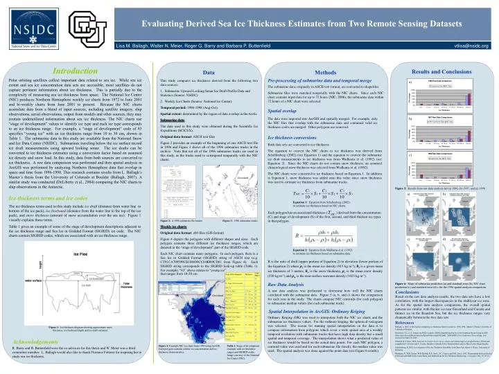
Evaluating Derived Sea Ice Thickness Estimates from Two Remote Sensing Datasets

1. Evaluating Derived Sea Ice Thickness Estimates from Two Remote Sensing Datasets Lisa M. Ballagh, Walter N. Meier, Roger G. Barry and Barbara P. Buttenfield vtlisa@nsidc.org Introduction Results and Conclusions Data Methods Polar orbiting satellites collect important data related to sea ice. While sea ice extent and sea ice concentration data sets are accessible, most satellites do not capture pertinent information about ice thickness. This is partially due to the complexity of measuring sea ice thickness from space. The National Ice Center (NIC) produces Northern Hemisphere weekly ice charts from 1972 to June 2001 and bi-weekly charts from June 2001 to present. Because the NIC charts assimilate data from a blend of input sources, including satellite imagery, ship observations, aerial observations, output from models and other sources, they may contain underutilized information about sea ice thickness. The NIC charts use “stage of development” values to identify ice type and each ice type corresponds to an ice thickness range. For example, a “stage of development” code of 83 specifies “young ice” with an ice thickness range from 10 to 30 cm, shown in Table 1. The submarine data in this study are available from the National Snow and Ice Data Center (NSIDC). Submarines traveling below the ice surface record ice draft measurements using upward looking sonar. The ice drafts can be converted to ice thickness estimates using a conversion factor based on assumed ice density and snow load. In this study, data from both sources are converted to ice thickness. A raw data comparison was performed and then spatial analysis in ArcGIS was performed by analyzing Northern Hemisphere data that overlap in space and time from 1996-1998. This research contains results from L. Ballagh’s Master’s thesis from the University of Colorado at Boulder (Ballagh, 2007). A similar study was conducted (DeLiberty et al., 2004) comparing the NIC charts to ship observations in the Antarctic. Pre-processing of submarine data and temporal merge • This study compares ice thickness derived from the following two data sources: • Submarine Upward Looking Sonar Ice Draft Profile Data and Statistics (Source: NSIDC) • Weekly Ice Charts (Source: National Ice Center) • Temporal period: 1996-1998 (Aug-Oct) • Spatial extent: determined by the region of data overlap in the Arctic • Submarine data • The data used in this study were obtained during the Scientific Ice Expeditions (SCICEX). • Original data format: ASCII text files • Figure 2 provides an example of the beginning of one ASCII text file in 1996 and Figure 3 shows all of the 1996 submarine tracks in the archive. Note that not all of the 1996 submarine tracks are used in this study, as the tracks need to correspond temporally with the NIC charts. • Figure 2: A 1996 submarine file header Figure 3: 1996 submarine tracks • Weekly ice charts • Original data format: e00 files (GIS format) • Figure 4 depicts the polygons with different shapes and sizes. Each polygon contains three different ice thickness ranges, which are denoted in the “stage of development” part of the SIGRID code. • Each NIC chart contains many polygons. In each polygon, there is a Sea Ice in Gridded Format (SIGRID) string of ASCII text (e.g. CT91CA709599CB108699CC018399CD81 from Figure 4). Each SIGRID string corresponds to the SIGRID look-up table (Table 1). For example, “83” above relates to “young ice” a) The submarine data, originally in ASCII text format, are converted to shapefiles. Submarine files were matched temporally with the NIC charts. Since each NIC chart contains input data for up to 72 hours (NIC, 2006), the submarine data within 72 hours of a NIC chart were selected. Spatial overlap The data were imported into ArcGIS and spatially merged. For example, only the NIC files that overlap with the submarine data and contained valid ice thickness codes are merged. Other polygons are removed. b) Ice thickness conversions Both data sets are converted to ice thickness. The equation to convert the NIC charts to ice thickness was derived from Schellenberg (2002) (see Equation 1) and the equation to convert the submarine ice draft measurements to ice thickness was from Wadhams et al. (1992) (see Equation 2). Since the NIC charts do not contain snow thickness, an assumed climatological snow thickness was selected from Wadhams et al. (1992). The NIC charts were converted to ice thickness based on Equation 1. In addition to Equation 1, snow thickness was added onto this value since snow thickness was used to estimate ice thickness from submarine tracks. c) Greenland Figure 5: Results from raw data analysis for (a) 1996, (b) 1997, and (c) 1998. a) b) Ice thickness terms and ice codes Equation 1: Equation from Schellenberg (2002) to estimate ice thickness based on NIC charts. The ice thickness terms used in this study include ice draft (distance from water line to bottom of the ice pack), ice freeboard (distance from the water line to the top of the ice pack), and snow thickness (amount of snow accumulation over the sea ice). Figure 1 visually explains these terms. Table 1 gives an example of some of the stage of development descriptions adjacent to the ice thickness range and Sea Ice in Gridded Format (SIGRID) ice code. The NIC charts contain SIGRID codes, which are associated with an ice thickness range. Each polygon has an associated thickness ( ) derived from the concentration (C) and stage of development (S) of the first, second, and third thickest ice types in that polygon. c) d) Equation 2: Equation from Wadhams et al. (1992) to estimate ice thickness based on submarine data. R is the ratio of draft (upper portion of Equation 2) to elevation (lower portion of the Equation 2) where ρi is the mean ice density (915 kg m-3), hiis a given mean ice thickness of 3 meters, hs is the snow thickness, ρs is the mean snow density (330 kg m-3) and ρw is the near-surface seawater density (1023 kg m-3). that ranges from 10-30 cm. Raw Data Analysis Figure 6: Maps of submarine prediction (a) and standard error (b), NIC chart prediction (c) and standard error (d) c for the 1996 spatial analysis comparison. A raw data analysis was performed to determine how well the NIC charts correlated with the submarine data. Figure 5 (a, b, and c) shows the comparison for each year in the study. The charts compare NIC centroids (for each polygon) to submarine median values (for each submarine track). Conclusions Greenland Based on the raw data analysis results, the two data sets have a low correlation, with the largest discrepancies in the multiyear ice zone. As for the spatial data analysis comparison, the overall spatial patterns are similar, with thicker ice near Greenland and Canada and thinner ice in the Beaufort Sea, but the ice thickness ranges vary dramatically between the two data sets. Spatial Interpolation in ArcGIS: Ordinary Kriging Ordinary Kriging (OK) was used to interpolate both the NIC ice charts and the submarine ice thickness values. For the ordinary kriging, the spherical variogram was selected. The reason for running spatial interpolation on the data is to compare information from polygons which cover a wide spatial area at a weekly temporal resolution with submarine tracks that have high data density but a small spatial and temporal coverage. The interpolation shows what a predicted value of ice thickness would be based on the actual data points. For each NIC polygon, a centroid value was used and for each submarine file (track), the median value was used. The spatial analysis was done against the point data (see Figure 6 results). References Ballagh, L. 2007. A first look at comparing ice thickness from two sources, 1996-1998. Master’s Thesis, University of Colorado at Boulder. DeLiberty, T.L., C.A. Geiger, and M.D. Lemcke (2004), Quantifying Sea Ice in the Southern Ocean Using ArcGIS (http://gis.esri.com/library/userconf/proc04/docs/pap1965.pdf). 2004 ESRI's User Conference Proceedings. Last accessed on April 10, 2006. National Ice Center. 2006. National Ice Center Arctic sea ice charts and climatologies in gridded format. Edited and compiled by F. Fetterer and C. Fowler. Boulder, Colorado USA: National Snow and Ice Data Center. Digital media. Schellenberg, B. 2002. Investigation of Sea-Ice Thickness Variability in the Ross Sea. Master’s Thesis, University of Delaware. Wadhams, P., W.B. Tucker, W.B. Krabill, R.N. Swifc, J.C. Comiso and N.R. Davis, 1992. Relationship between Sea Ice Freeboard and Draft in the Arctic Basin, and Implications for Ice Thickness Monitoring. J. Geophys. Res., 97 (C12). Figure 1: Ice thickness diagram showing approximate snow thickness, ice freeboard depth and ice draft variation. Acknowledgements Figure 4: Example NIC ice chart from 1996 using ArcGIS. Each polygon contains similar ice concentration and ice thickness characteristics. Table 1: Stage of development example with ice thickness ranges and SIGRID codes. Image courtesy of the National Ice Center (NIC). R. Barry and B. Buttenfield were the co-advisors for this thesis and W. Meier was a third committee member. L. Ballagh would also like to thank Florence Fetterer for inspiring her to study sea ice thickness.