Download
1 / 40
510 likes | 978 Views
An Introduction of Image Segmentation. 主講者 : 陳建齊. Outline & Content. Introduction Thresholding Edge-based segmentation Region-based segmentation conclusion. Introduction. What is segmentation? Three major ways to do. Thresholding Edge-based segmentation Region-based segmentation.

E N D
Outline & Content • Introduction • Thresholding • Edge-based segmentation • Region-based segmentation • conclusion
Introduction • What is segmentation? • Three major ways to do. • Thresholding • Edge-based segmentation • Region-based segmentation
Thresholding • Finding histogram of gray level intensity. • Basic Global Thresholding • Otsu’s Method • Multiple Threshold • Variable Thresholding
Edge-based segmentation • Using mask to detect edge in image by convolution. • Basic Edge Detection • The Marr-Hildreth edge detector(LoG) • Short response Hilbert transform(SRHLT) • Watersheds
Region-based segmentation • Finding region, but not finding edge. • Region Growing • Data Clustering (Hierarchical clustering) • Partitional clustering • Cheng-Jin Kuo`s method
ThresholdingBasic Global Thresholding • Select an initial To • Segment image use: • Compute the average intensity and for the pixels in and . • Compute a new threshold: • Until the difference between values of T is smaller than a predefined parameter.
Otsu’s Method • {0,1,2,…,L-1} , L means gray level intensity M*N is the total number of pixel. denote the number of pixels with intensity • we select a threshold , and use it to classify : intensity in the range and : • , • , • , it is global variance.
it is between-class variance • , it is a measure of separability between class. For x = 0,1,2,…,M-1 and y = 0,1,2…,N-1. • Using image Smoothing/Edge to improve Global Threshold
Multiple Threshold • As Otsu’s method, it takes more area and k* • Disadvantage: it becomes too complicate when number of area more than three.
Variable Thresholding • Image partitioning . • It is work when the objects of interest and the background occupy regions of reasonably comparable size. If not , it will fail.
Variable thresholding based on local image properties • Let and denote the standard deviation and mean value of the set of pixels contained in a neighborhood, .
Using moving average • It discussed is based on computing a moving average along scan lines of an image. • denotethe intensity of the point at step k+1. n denote the number of point used in the average. • is the initial value. • ,where b is constant and is the moving average at point(x,y)
Edge-based segmentationBasic Edge Detection • Why we can find edge by difference? • image intensity first-order deviation second-order deviation
Gradient • The image gradient is to find edge strength and direction at location (x,y) of image. • The magnitude (length) of vector , denoted as M(x,y): • The direction of the gradient vector is given by the angle:
Roberts cross-gradient operators: • Prewitt operator: • Sobel operator:
The Marr-Hildreth edge detector(LoG) • This is second-order deviation, we call Laplacian. • Filter the input image with an n*n Gaussian lowpass filter. 99.7% of the volume under a 2-D Gaussian surface lies between about the mean. So .
Short response Hilbert Transform(SRHLT) • Hilbert transform • ,
Watersheds • Algorithm: • , g(s,t) is intensity. n= min+1 to n = max +1. And let T[n]=0, others 1. • , is minimum point beneath n.
Markers • External markers: • Points along the watershed line along highest points. • Internal markers: (1) That is surrounded higher points . (2) Points in region form a connected component (3) All points in connected component have the same intensity.
Region-based segmentationRegion Growing • Algorithm: • Choose a random pixels • Use 8-connected and threshold to determine • Repeat a and b until almost points are classified.
Simulation of region growing (90% pixels ) Threshold/second: 20/4.7 seconds.
Data Clustering • Using centroid to represent the huge numbers of clusters • Hierarchical clustering, we can change the number of cluster anytime during process if we want. • Partitional clustering , we have to decide the number of clustering we need first before we begin the process.
Hierarchical clustering • Algorithm of hierarchical agglomeration(built): • See every single data as a cluster . • Find out , for the distance is the shortest. • Repeat the steps until satisfies our demand. • as the distance between data a and b
Algorithm of hierarchical division(break up ): • Diameter of cluster
See the whole database as one cluster. • Find out the cluster having the biggest diameter • , . • Split out x as a new cluster , and see the rest data points as . • If > , then split yout of and classify it to • Back to step2 and continue the algorithm until and is not change anymore.
Partitional clustering • Decide the numbers of the cluster(k-means) • Problem: • Initial problem
Number of regions are more than clusters you set. • Determine the number of clusters.
Simulation of k-means Clustering/time: 9 clustering/ 0.1
Cheng-Jin Kuo`s method • Algorithm
Adaptive threshold decision with local variance • Variance of Lena: 1943 • Small variance cause small threshold.
Adaptive threshold decision with local variance and frequency • Variance of baboon: 1503
High frequency, high variance. Set highest threshold. (4,1) • High frequency, low variance. Set second high threshold. (4,2) • Low frequency, high variance. Set third high threshold. (1,4) • Low frequency, low variance. Set the lowest threshold. • (1,1)
Conclusion • Speed • Connectivity • System reliability
Reference • R. C. Gonzalez, R. E. Woods, Digital Image Processing third edition, Prentice Hall, 2010. • C. J. Kuo, J. J. Ding, Anew Compression-Oriented Fast image Segmentation Technique, NTU,2009.