Download
1 / 42
420 likes | 679 Views
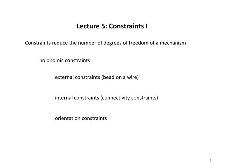
Lecture 5: Constraints I. Constraints reduce the number of degrees of freedom of a mechanism. holonomic constraints. external constraints (bead on a wire). internal constraints (connectivity constraints). orientation constraints.

E N D
Lecture 5: Constraints I Constraints reduce the number of degrees of freedom of a mechanism holonomic constraints external constraints (bead on a wire) internal constraints (connectivity constraints) orientation constraints
Holonomic constraints can be written in terms of the coordinates Simple holonomic constraints are linear in the coordinates Nonsimple holonomic constraints are nonlinear in the coordinates (I will address nonholonomic constraints in Lecture 7.)
Bead on a wire I call it a bead, and I’ll treat it as a point — three degrees of freedom mg
A little digression on the properties of curves in space the tangent vector This is the unit tangent vector we’ll do a lot with nonunit tangent vectors
Bead on a wire Curve is defined by a parameterization arclength general parameter
Bead on a wire Kinetic energy add in the potential energy and write the Lagrangian
Bead on a wire The only variable here is c (a proxy for s), so we build one EL equation
Bead on a wire The Euler-Lagrange equation
Bead on a wire We can solve this analytically in the simple case where is a constant. The helix is such a case
Bead on a wire so the Euler-Lagrange equation is which is easily integrated to give
Bead on a wire From which we obtain
Bead on a wire The force on the bead from the wire
Bead on a (complicated) wire wire profile
Bead on a (complicated) wire This one has to be done numerically Constraints are from the previous slide x y z
Bead on a (complicated) wire The constrained Lagrangian The Euler-Lagrange equation Make two first order equations out of this
Bead on a (complicated) wire The maximum height of the track is unity at c = 0 Starting from rest below unity leads to an oscillation Starting at c= 0 with no motion gives (unstable) equilibrium Add motion and we get a roller coaster-like motion Let’s look at the Mathematica code
Bead on a (complicated) wire The Lagrangian, the Euler-Lagrange equations and the partition into two equations The Euler-Lagrange equation
Bead on a (complicated) wire The odes, the initial conditions and a space for the answer
Bead on a (complicated) wire The solution procedure and the answers
Bead on a (complicated) wire RESULTS Start from c = 0 and u =0.1 and let 0 ≤ t ≤ 8π This gives several runs around the track We can look at speed vs. time height vs. time energy vs. time (conserved)
Bead on a (complicated) wire height
Bead on a (complicated) wire energy
Bead on a (complicated) wire speed vs.height initial speed is 0.1
Link on a wire I will eventually specialize to an axisymmetric link on the helical wire, but we can say some general things first I will align the K axis of the link with the local curve
Link on a wire I suppose the link to be small enough that I can neglect the curvature of the wire locally, so I can still impose the position constraints But now I have an orientation constraint
Link on a wire divide lhs by sinq We have determined two Euler angles: f and q We are left with y, and the system has two degrees of freedom
Link on a wire Doing this in general is really difficult and it will obscure what is going on in a sea of algebra so let’s stick to the helix
Link on a wire Start by letting f = c, which is almost intuitive sinq needs to be proportional to –a cosq needs to be proportional to -h
Link on a wire Two degrees of freedom — c and y— as we noted before If the link is axisymmetric this problem has a closed from solution! I’m going to leave this as a problem for you
We’ve been looking at external constraints on a single link I’d like to start on internal constraints connecting links I will split these into orientation constraints and connectivity constraints I will also split them into simple and nonsimple constraints Orientation constraints are often simple Connectivity constraints are usually nonsimple
Some notation I’m going to work, for now, with fairly symmetric bodies their centers of mass are also their “actual center” rectangular solids cylinders ellipsoids . . . . I will use body coordinates parallel to the principal moments I will usually (at least for now) connect bodies at their ends and suppose the ends to be in the K direction
I suppose the semiaxes to be a, b and c in the I, J and K directions Here b = a. The connectivity of these two links relates the center of mass of link two to the center of mass of link one This relates x2, y2 and z2 to the coordinates of link 1 and all six Euler angles It’s a connectivity constraint and it is not simple it is nonsimple — by which I mean not linear
The system has nine degrees of freedom It started with twelve and we took three out You can see that substituting this into the Lagrangian will lead to quite a mess It gets worse as we add links We’re going to learn cool ways to deal with this, but not just yet
We can further constrain this system by attaching the first link to the ground at the origin of the inertial system and this system now has six degrees of freedom
Suppose the two links we looked at to be connected by a hinge instead of a magic spherical joint Here I denotes the common I vector for both links the direction of the hinge pin
and these will be equal if (It is possible to have a more complicated hinge relation and we may get to that near the end of the course or we may not.)
Think about this operationally We rotate both of these through the same f angle Then we rotate each about a different q angle We do not rotate either about its y angle