Download
1 / 38
390 likes | 593 Views
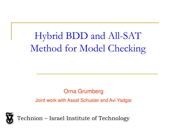
Hybrid BDD and All-SAT Method for Model Checking. Orna Grumberg Joint work with Assaf Schuster and Avi Yadgar. Technion – Israel Institute of Technology. Contribution of this Work. Hybrid All-SAT and BDD model checking Exploit the strength of each method. Avoid drawbacks of both methods.

E N D
Hybrid BDD and All-SAT Method for Model Checking Orna Grumberg Joint work with Assaf Schuster and Avi Yadgar Technion – Israel Institute of Technology
Contribution of this Work • Hybrid All-SAT and BDD model checking • Exploit the strength of each method. • Avoid drawbacks of both methods. • Dual representation for All-SAT solving • Exploit efficient SAT procedures. • bcp(), conflict driven learning. • Extract information from the structure of a model. • Simplify and speedup the All-SAT solving process • Minimize the representation of solutions.
Model Checking – Pre-image Computation • Pre-image(S) – The set of predecessors of states in S. • - state variables, - input variables. • - Transition Relation. • - set of states.
Model Checking • Checking of a safety property AGp: Input for the algorithm is S0,Tr and P. • Start with the error states. • Iteratively look for states in S0.
Model Checking • Requires operations on sets • Union, intersection, and quantification. • Common representation of sets: BDDs • Union and intersection - polynomial in the size of the BDDs. • Quantification – exponential in the size of the BDD. • Explosion of intermediate results during pre-image computation.
All-SAT Pre-image Computation • Each solution describes: • A current-state not in . • A valid transition. • A next-state in new. • We need all the solutions which differ in the assignment to . • Represent different current-states.
Model Checking – Hybrid Method • Use BDD operations for all but pre-image computation
All-SAT – Blocking Clauses • Find allthe satisfying assignments(solutions) of a formula. • Extend the SAT algorithm: • Create a clause to block each solution found. • Resume search with the new clause added. • Common in All-SAT tools. • Direct and simple, natural for the solver. • Disadvantage: • Rapid space growth of the solver.
X3 X5 0 1 X1 All-SAT – Blocking BDDs [Gupta et al] • A partial assignment A agrees with a BDD B if there is a path from the root of B to the node ‘1’. • Values of the nodes in the path correspond to A. • A1: x1=1,x8=0. • A2: x1=0,x5=1 • A3: x3=0,x5=0 1 0 0 1 0 1
All-SAT – Blocking BDDs • Restrict the search space of a SAT solver by a BDD B. • Check if the current partial assignment agrees with B each time variables from B are assigned. • Backtrack if the assignment does not agree. • Use for All-SAT • Add each solution to a BDD S. • Force agreement with S.
Our Hybrid Pre-image computation • Look for all the assignments to which can be extended to a solution for: • newand S*are given as BDDs. • Restrict the search by the BDD of ¬S*. • new will be discussed later. • Tris in CNF. • Return a BDD of the solutions • Its negation is used for blocking known solutions.
All-SAT Decision Heuristic • Add a graph representation of the transition relation to the All-SAT solver. • Use information from the graph for making decisions in the All-SAT solver. • Find sets of solutions instead of single ones. • Compute dynamic transition relation. • Detect independent sub-problems. • Reduce sub-problems to SAT.
Transition Relation Graph (TRG) v3 Partitioned Transition Relation: x’2 x’1 v1 v2 v1 v2 v3 • x’: next-state • x: current-state • i: input • v: intermediate i1 i2 X2 i3 X1
Transition Relation Graph • The intermediate variables exists in the CNF representation of Tr. • The operator of a variable is represented by a set of clauses:
TRG – Justification • Assignment to a node can be justified by its successors. x’2 x’1 v2 v1=0 v3 v3=0 i1 i2 X1 X2 i3
All-SAT TRG-Based Decision • Decision i+1 justifies decision i. • If not needed –justify a new root. • If all roots are justified – a solution was found. x’2=1 x’1=1 v2=1 v2 v1 v3 • Backtrack to change the value of at least one current state variable. i1 i2 X1 X2=0 X2=1 X2 i3 i1=1 i2=1
All-SAT TRG-Based Decision • A solution is a justification of an assignment to the roots. • Represents a set of current states. • Less instantiations of assignments. • Each assignment is instantiated more quickly. • Smaller representation of the solutions.
All-SAT TRG-Based Decision • Values of the roots – all the assignments in new x’1 TRG x’2 x’4 x’1 x’3 x’1=0 x’4=0 x’3=0 x’2=0 x’1=1 x’3 x’2 x’4 1 0
All-SAT TRG-Based Decision • A solution is a justification of an assignment to the roots. • Represents a set of current states. • Less instantiations of assignments. • Each assignment is instantiated more quickly. • Smaller representation of the solutions. • DFS over the BDD of new • Handle sets of assignments from new at once. • Avoid repetition of justifications.
All-SAT TRG-Based Decision • Computes sets of current states (justifications) for each subset of new • Unlike All-SAT which handles a single assignment at a time • Unlike BDDs that can compute the set of all current states for new at once
All-SAT optimizations • Independent Roots • Determined statically or dynamically. • Sub-problems can be solved independently. x’2 x’2=1 x’1 v2 v1 v3 i1 i2 X2 i3 i1=1 X1
All-SAT optimizations • Non-important roots • Determined statically or dynamically. • Reduce sub-problems to SAT. x’2 x’2=1 x’1 v2 v1 v3 i2 X2 x’2=1 i3 X3 X1
Hybrid Model Checking – Final Notes • Dynamic transition relation • Only variables of each path in the BDD of new are justified. • Incremental learning of the All-SAT solver • Learning is independent of the current iteration.
Experimental Results • Experiments were done on ISCAS89 and ISCAS99 benchmarks • 50~6000 state variables • Compared to a BDD model checker • Results are not consistent for all models • For each model, one method constantly performed better than the other. • For most models memory requirements is lower.
Experimental Results • On “good” examples, less time is spent on quantification and more on Boolean operations • Quantification is faster • Independent Roots and Non-Important Roots enhance performance.
Conclusion • Hybrid All-SAT and BDD model checking • Exploit the strength of each method. • Avoid drawbacks of both methods. • Dual representation All-SAT solving • Exploit efficient SAT procedures. • bcp(), conflict driven learning. • Extract information from the structure of a model. • Simplify and speedup the All-SAT solving process • Minimize the representation of solutions.
Extensions • Parallel All-SAT model checking • Adaptation of All-SAT solver for general All-SAT problems. • Optimizations of the current All-SAT scheme for model checking
Parallel All-SAT Model Checking • Distribute the pre-image computation. • Split the space of solutions into windows. • A window is represented by a partial assignment to the current-state variables. • A solution is an extension to the partial assignment of the window. • Split the space to as many subspaces as needed for maintaining CPU load balance.
Parallel All-SAT Model Checking • Each node only instantiates solutions in its window. Split S* according to the window. • Reduce the space requirement of a node. • Prefer memory load balance over CPU load balance.
Parallel All-SAT Model Checking • Init • Find solutions in window • Merge new for next iteration.
Parallel All-SAT Model Checking • Use conflict clauses incrementally. • Share conflict clauses among nodes. • Adapt to grid computation.
TRG for General All-SAT • Extract a ‘circuit-like’ structure from general CNF formulae. • Gain more information about the formulae. • Incorporate additional information into the TRG, according to the type of problem being solved.
v1 v2 v3 v4 TRG for General All-SAT • Extract a ‘circuit-like’ structure from general CNF formulae. a d c b e
Optimizations – Early Quantification in BDD • For a partitioned transition relation and an order f1…fn, define • Order the functions such that fi+1 shares the most current state variables with f1..fi. • Group related variables
Optimizations – Early Quantification in the Hybrid method • Assign and justify the roots of the TRG (next-state variables) in the order determined by early quantification • Order the variables in the BDD new accordingly
Optimizations – Success Learning • Store the set of solutions for a cut. x’1=0 x’1=0 v2=0 v2 v1 v1=0 v3=0 v3=0