Download
1 / 15
150 likes | 310 Views
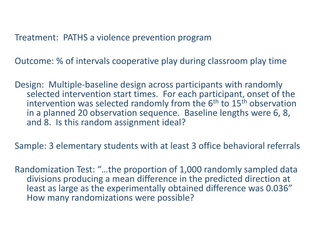
Treatment: PATHS a violence prevention program Outcome: % of intervals cooperative play during classroom play time

E N D
Treatment: PATHS a violence prevention program Outcome: % of intervals cooperative play during classroom play time Design: Multiple-baseline design across participants with randomly selected intervention start times. For each participant, onset of the intervention was selected randomly from the 6th to 15th observation in a planned 20 observation sequence. Baseline lengths were 6, 8, and 8. Is this random assignment ideal? Sample: 3 elementary students with at least 3 office behavioral referrals Randomization Test: “…the proportion of 1,000 randomly sampled data divisions producing a mean difference in the predicted direction at least as large as the experimentally obtained difference was 0.036” How many randomizations were possible?
Computational Example Bob? Candy? Abbey? Dave? Bob? Candy? Abbey? Dave? Bob? Candy? Abbey? Dave? Bob? Candy? Abbey? Dave? Session
Randomization The baselines were chosen to last 4, 8, 12, and 16 sessions, and participants were randomly assigned to baseline lengths. It turned out that Bob, Candy, Abbey, and Dave had baseline lengths of 4, 8, 12 and 16, respectively. Bob Candy Abbey Dave
Data Session 1 2 3 4 5 6 7 8 9 10 11 12 13 14 15 16 17 18 19 20 Bob 8 7 6 7 4 5 6 5 4 4 5 2 4 3 4 5 4 3 2 2 Candy 6 7 8 7 5 7 6 8 6 5 4 4 4 3 2 5 3 4 3 6 Abbey 5 5 4 6 4 5 6 7 4 5 6 5 2 3 2 4 1 0 2 3 Dave 8 6 7 7 8 5 7 8 7 6 7 8 5 6 8 8 6 4 4 5
Randomization Distribution The randomization distribution is composed of the test statistic values from all possible assignments given the randomization scheme We have computed 2, we have 22 to go
p-value The p-value is the proportion of values in the randomization distribution that are as large or larger than the obtained test statistic value. If we calculate W for all 24 randomizations we will find that the largest value is 11.022, which is the obtained test statistic value
SAS syntax prociml; x={87674565445243454322, 67875768654443253436, 55464567456523241023, 86778578767856886445}; p1init=4; p2init=8; p3init=12; p4init=16; p1fin=p1init+1; p2fin=p2init+1; p3fin=p3init+1; p4fin=p4init+1;
ncases=nrow(x); nobs=ncol(x); a1o=sum(x[1,1:p1fin-1])/(p1fin-1); b1o=sum(x[1,p1fin:nobs])/(nobs-p1fin+1); a2o=sum(x[2,1:p2fin-1])/(p2fin-1); b2o=sum(x[2,p2fin:nobs])/(nobs-p2fin+1); a3o=sum(x[3,1:p3fin-1])/(p3fin-1); b3o=sum(x[3,p3fin:nobs])/(nobs-p3fin+1); a4o=sum(x[4,1:p4fin-1])/(p4fin-1); b4o=sum(x[4,p4fin:nobs])/(nobs-p4fin+1); test1ob=(a1o-b1o)+(a2o-b2o)+(a3o-b3o)+(a4o-b4o);
counter1=0; count1=0; do i=1 to 4; xperm=x[i,]; if i=1 then xx=x[2:4,]; if i=2 then xx=x[1,]//x[3:4,]; if i=3 then xx=x[1:2,]//x[4,]; if i=4 then xx=x[1:3,]; do j=1 to 3; xperm1=xperm//xx[j,]; if j=1 then xxx=xx[2:3,]; if j=2 then xxx=xx[1,]//xx[3,]; if j=3 then xxx=xx[1:2,]; do k=1 to 2; xperm2=xperm1//xxx[k,]; xxxx=xxx[3-k,]; xperm3=xperm2//xxxx; counter1=counter1+1;
a1=sum(xperm3[1,1:p1fin-1])/(p1fin-1); b1=sum(xperm3[1,p1fin:nobs])/(nobs-p1fin+1); a2=sum(xperm3[2,1:p2fin-1])/(p2fin-1); b2=sum(xperm3[2,p2fin:nobs])/(nobs-p2fin+1); a3=sum(xperm3[3,1:p3fin-1])/(p3fin-1); b3=sum(xperm3[3,p3fin:nobs])/(nobs-p3fin+1); a4=sum(xperm3[4,1:p4fin-1])/(p4fin-1); b4=sum(xperm3[4,p4fin:nobs])/(nobs-p4fin+1); testst1=(a1-b1)+(a2-b2)+(a3-b3)+(a4-b4); diff1=a1-b1; diff2=a2-b2; diff3=a3-b3; diff4=a4-b4; if testst1>=test1ob then count1=count1+1; pvalue1=count1/counter1; print testst1 diff1 diff2 diff3 diff4; end; end; end; print test1ob; print pvalue1; quit iml;
TESTST1 DIFF1 DIFF2 DIFF3 DIFF4 11.020833 3.125 2.6666667 3.0416667 2.1875 10.104167 3.125 2.6666667 1.25 3.0625 9.8125 3.125 2.1666667 2.3333333 2.1875 7.9791667 3.125 2.1666667 1.25 1.4375 9.3541667 3.125 0.8333333 2.3333333 3.0625 8.4375 3.125 0.8333333 3.0416667 1.4375 10.041667 2.3125 2.5 3.0416667 2.1875 9.125 2.3125 2.5 1.25 3.0625 8.5416667 2.3125 2.1666667 1.875 2.1875 7.9166667 2.3125 2.1666667 1.25 2.1875 8.0833333 2.3125 0.8333333 1.875 3.0625 8.375 2.3125 0.8333333 3.0416667 2.1875 8.3333333 1.3125 2.5 2.3333333 2.1875 6.5 1.3125 2.5 1.25 1.4375 8.0416667 1.3125 2.6666667 1.875 2.1875 7.4166667 1.3125 2.6666667 1.25 2.1875 5.4583333 1.3125 0.8333333 1.875 1.4375 6.6666667 1.3125 0.8333333 2.3333333 2.1875 8.5208333 0.625 2.5 2.3333333 3.0625 7.6041667 0.625 2.5 3.0416667 1.4375 8.2291667 0.625 2.6666667 1.875 3.0625 8.5208333 0.625 2.6666667 3.0416667 2.1875 6.1041667 0.625 2.1666667 1.875 1.4375 7.3125 0.625 2.1666667 2.3333333 2.1875 TEST1OB 11.020833 PVALUE1 0.0416667
Software Options SCRT-R An R Package for the nonparametric analysis and meta-analysis of single-case experimental data https://perswww.kuleuven.be/~u0053535/ Bulte, I, & Onghena, P. (2008). An R package for single-case randomization tests. Behavioral Research Methods, 40, 467- 478. Bulte, I., & Onghena, P. (2009). Randomization tests for multiple- baseline designs: An extension of the SCRT-R package. Behavior Research Methods, 41, 477-485.