Download
1 / 47
480 likes | 615 Views
Proteiinianalyysi 4. Piilomarkovmallit http://www.bioinfo.biocenter.helsinki.fi/downloads/teaching/spring2006/proteiinianalyysi. Alignment of sequences with a structure: hidden Markov models. Hidden Markov Models. HMMs suit well on describing correlation among neighbouring sites

E N D
Proteiinianalyysi 4 Piilomarkovmallit http://www.bioinfo.biocenter.helsinki.fi/downloads/teaching/spring2006/proteiinianalyysi
Alignment of sequences with a structure: hidden Markov models Hidden Markov Models • HMMs suit well on describing correlation among neighbouring sites • probabilistic framework allows for realistic modelling • well developed mathematical methods; provide • best solution (most probable path through the model) • confidence score (posterior probability of any single solution) • inference of structure (posterior probability of using model states) • we can align multiple sequence using complex models and simultaneously predict their internal structure
Coin game • Fair coin: p(1)=p(0)=0.5 • 01110001101011100… • Biased coin: p(1)=0.8, p(0)=0.2 • 111011111100100111… • Observed series: 010111001010011 • P(fair coin)=0.515 • P(biased coin)=0.880.27 • P(biased coin)/P(fair coin)=0.07
Multiple sequence alignment (msa) • A) define characters for phylogenetic analysis • B) search for additional family members SeqA N ∙FLS SeqB N∙ F – S SeqC NKYLS SeqD N ∙ YLS NYLSNKYLSNFSNFLS +K -L YF
Markov process • State depends only on previous state • Markov models for sequences • States have emission probabilities • State transition probabilities
piilomarkovmalli (HMM) • probabilistinen malli aikasarjoille tai lineaarisille sekvensseille • puheentunnistuksessa • proteiiniperheiden mallitus • kuvaa todennäköisyysjakaumaa sekvenssiavaruuden yli • todennäköisyyksien summa = 1 • generatiivinen malli • sekvenssi voidaan linjata ja ”pisteyttää” mallia vastaan
Piilomarkovmalli kaksitilamuuttujalle t(1,1) t(2,2) t=transitiotodennäköisyys p=emissiotodennäköisyys t(1,2) t(2,end) end 1 HMM 2 p1(a) p1(b) p2(a) p2(b) tila, p 1 1 2 end a b a havaittu symbolisekvenssi, x t(1,1) t(1,2) t(2,end) p1(a) p1(b) p2(a) P(x,p | HMM)
profiili-HMM insert match delete 2 begin 1 end 3 4 match state emits one of 20 amino acids insert state emits one of 20 amino acids delete, begin, end states are mute
profiili-HMM • lineaarinen malli • pisteytys vastaa log-odds-scorea • aukkosakkokin muodollisesti a+b(x-1) • käyttö: • monen sekvenssin linjaus • homologien tunnistaminen: millä todennäköisyydellä HMM generoi testisekvenssin • sekvenssin linjaus mallia vastaan
HMM with multiple paths through the model for ACCY. The highlighted path is only one of several possibilities.
Viterbi algorithm • computes the sequence scores over the most likely path rather than over the sum of all paths.
Forward algorithm • Similar to Viterbi except that a sum rather than the maximum is computed
What the Score Means Once the probability of a sequence has been determined, its score can be computed. Because the model is a generalization of how amino acids are distributed in a related group (or class) of sequences, a score measures the probability that a sequence belongs to the class. A high score implies that the sequence of interest is probably a member of the class, and a low score implies it is probably not a member.
Optimisation • The Baum-Welch algorithm is a variation of the forward algorithm described earlier. It begins with a reasonable guess for an initial model and then calculates a score for each sequence in the training set over all possible paths through this model . During the next iteration, a new set of expected emission and transition probabilities is calculated. The updated parameters replace those in the initial model, and the training sequences are scored against the new model. The process is repeated until model convergence, meaning there is very little change in parameters between iterations. • The Viterbi algorithm is less computationally expensive than Baum-Welch.
Heuristics • There is no guarantee that a model built with either the Baum-Welch or Viterbi algorithm has parameters which maximize the probability of the training set. As in many iterative methods, convergence indicates only that a local maximum has been found. Several heuristic methods have been developed to deal with this problem.
Heuristics: parallel trials • start with several initial models and proceed to build several models in parallel. When the models converge at several different local optimums, the probability of each model given the training set is computed, and the model with the highest probability wins.
Heuristics: add noise • add noise, or random data, into the mix at each iteration of the model building process. Typically, an annealing schedule is used. The schedule controls the amount of noise added during each iteration. Less and less noise is added as iterations proceed. The decrease is either linear or exponential. The effect is to delay the convergence of the model. When the model finally does converge, it is more likely to have found a good approximation to the global maximum.
Overfitting and regularization CGGSLLNAN--TVLTAAHC CGGSLIDNK-GWILTAAHC CGGSLIRQG--WVMTAAHC CGGSLIREDSSFVLTAAHC
Dirichlet mixtures • A sophisticated application of this method is known as Dirichlet mixtures. The mixtures are created by statistical analysis of the distribution of amino acids at particular positions in a large number of proteins. The mixtures are built from smaller components known as Dirichlet densities. • A Dirichlet density is a probability density over all possible combinations of amino acids appearing in a given position. It gives high probability to certain distributions and low probability to others. For example, a particular Dirichlet density may give high probability to conserved distributions where a single amino acid predominates over all others. Another possibility is a density where high probability is given to amino acids with a common identifying feature, such as the subgroup of hydrophobic amino acids. • When an HMM is built using a Dirichlet mixture, a wealth of information about protein structure is factored into the parameter estimation process. The pseudocounts for each amino acid are calculated from a weighted sum of Dirichlet densities and added to the observed amino acid counts from the training set. The parameters of the model are calculated as described above for simple pseudocounts.
Log-odds ratio • This number is the log of the ratio between two probabilities — the probability that the sequence was generated by the HMM and the probability that the sequence was generated by a nullmodel, whose parameters reflect the general amino acid distribution in the training sequences.
Limitations of profile-HMM • The HMM is a linear model and is unable to capture higher order correlations among amino acids in a protein molecule. • In reality, amino acids which are far apart in the linear chain may be physically close to each other when a protein folds. Chemical and electrical interactions between them cannot be predicted with a linear model. • Another flaw of HMMs lies at the very heart of the mathematical theory behind these models: the probability of a protein sequence can be found by multiplying the probabilities of the amino acids in the sequence. This claim is only valid if the probability of any amino acid in the sequence is independent of the probabilities of its neighbors. • In biology, this is not the case. There are, in fact, strong dependencies between these probabilities. For example, hydrophobic amino acids are highly likely to appear in proximity to each other. Because such molecules fear water, they cluster at the inside of a protein, rather than at the surface where they would be forced to encounter water molecules.
P=1 P=1 P=1 A simplified hidden Markov model (HMM) A 0.25 C 0.25 G 0.25 T 0.25 A 0.25 C 0.25 G 0.25 T 0.25 A 0.25 C 0.25 G 0.25 T 0.25 A 0.25 C 0.25 G 0.25 T 0.25 A 0.1 C 0.4 G 0.4 T 0.1 END BEGIN A 0.1 C 0.2 G 0.2 T 0.5 A 0.4 C 0.3 G 0.1 T 0.2 0.9 1.0 0.7 0.2 0.1
P=1 P=1 P=1 (a) Calculate the probability of the sequence TAG by following a path through the model’s three match states. A 0.25 C 0.25 G 0.25 T 0.25 A 0.25 C 0.25 G 0.25 T 0.25 A 0.25 C 0.25 G 0.25 T 0.25 A 0.25 C 0.25 G 0.25 T 0.25 A 0.1 C 0.4 G 0.4 T 0.1 END BEGIN A 0.1 C 0.2 G 0.2 T 0.5 A 0.4 C 0.3 G 0.1 T 0.2 0.9 0.7*0.5*0.7*0.4*0.7*0.4*0.9=0.0247 1.0 0.7 0.2 0.1
P=1 P=1 P=1 (b) Repeat a for a path that goes first to the insert state, then to a match state, then to a delete state, then to a match state and End. A 0.25 C 0.25 G 0.25 T 0.25 A 0.25 C 0.25 G 0.25 T 0.25 A 0.25 C 0.25 G 0.25 T 0.25 A 0.25 C 0.25 G 0.25 T 0.25 A 0.1 C 0.4 G 0.4 T 0.1 END BEGIN A 0.1 C 0.2 G 0.2 T 0.5 A 0.4 C 0.3 G 0.1 T 0.2 0.9 0.1*0.25*1*0.1*0.2*1*1*0.4*0.9=0.00018 1.0 0.7 0.2 0.1
(c) Which of the two paths is the more probable one, and what is the ratio of the probability of the higher to the lower one? • p(path1)/p(path2) = 0.0247 / 0.00018 = 137.2 • The highest-scoring path is the best alignment of the sequence with the model. The Viterbi algorithm is similar to dynamic programming and finds the highest-scoring path.
Improving the model • Adjust the scores for the states and transition probabilities by aligning additional sequences with the model using an HMM adaptation of the expectation maximization algorithm. • In the expectation step, calculate all of the possible paths through the model, sum the scores, and then calculate the probability of each path. Each state and transition probability is then updated by the maximization step of the algorithm to make the model better predict the new sequence.
Information theory primer • Information, Uncertainty • Suppose we have a device that can produce 3 symbols, A, B, or C “uncertainty of 3 symbols” • Uncertainty = log2(M) with M being the number of symbols • Logarithm base 2 gives units in bits. • Example: In reading mRNA, if the ribosome encounters any one of 4 equally likely bases, then the uncertainty is 2 bits.
Surprisal u • Let symbols have probabilities Pi • Surprisal Ui = -log2(Pi) • For an infinite string of symbols, the average surprisal • H=S Piui = - S Pi log2 Pi (bits per symbol) • Sum over all symbols I • H is Shannon’s entropy
If all symbols are equally likely? • Hequiprobable = - S 1/M log2 (1/M) = log2 M
Coding • Shorter codes using few bits for common symbols and many bits for rare symbols. • M=4: A C G T with probabilities • P(A)=1/2, P(C)=1/4, P(G)=1/8, P(T)=1/8 • Surprisals U(A)=1 bit, U(C)=2 bits, U(G)=U(T)=3 bits • Uncertainty is H=1/2*1+1/4*2+1/8*3+1/8*3=1.75 (bits per symbol)
Recode symbols so that the number of binary digits equals the surprisal • A = 1 • C = 01 • G = 000 • T = 001 • The string ACATGAAC is coded as 1.01.1.001.000.1.1.01 • 14 / 8 = 1.75 bits per symbols
Noisy communication channels • Sender ----[noise]---- receiver • Two equally likely symbols sent at a rate of 1 bit per second • if x=0 is sent, probability of receiving y=0 is 0.99 and probability of receiving y=1 is 0.01, and vice versa • Then the uncertainty after receiving a symbol is Hy(x)=-0.99log20.99-0.01log20.01=0.081 • So the actual rate of transmission is R=1-0.081=0.919 bits per second
Information content of a scoring matrix by the relative entropy method (ignores background frequencies) • (a) calculate the entropy or uncertainty (Hc) for each column and for the entire matrix. Hc=-S pic log2(pic), where pic is the frequency of amino acid type i in column c. • Column 1: Hc=-(0.6 log2(0.6) + 2*0.1 log2(0.1)+0.2 log2(0.2))=1.571 • Column 2: Hc=-(0.7 log2(0.7) + 3*0.1 log2(0.1)=1.358 • Column 3: Hc=-(0.6 log2(0.6) + 2*0.1 log2(0.1)+0.2 log2(0.2))=1.571 • Column 4: Hc=-(0.7 log2(0.7) + 3*0.1 log2(0.1)=1.358 • Log2(x)=y y=log(x)/log(2)
(b) calculate the decrease in uncertainty or amount of information (Rc) for column 1 due to these data (for DNA, Rc=2-Hc and for proteins, Rc=4.32-Hc). • If it’s DNA: Rc=2-Hc =2-1.57=0.43 • If it’s protein: Rc=2-Hc =4.32-1.57=2.75
(c) calculate the amount that the uncertainty is reduced (or the amount of information contributed) for each base in column 1. • f(A)=0.6, HA,1=-0.6log2(0.6)=0.442 • f(G)=f(C)=0.1, HG,1= HC,1 =-0.1log2(0.1)=0.332 • f(T)=0.2, HT,1=-0.2log2(0.2)=0.464
Database searching • The first and most common operation in protein informatics...and the only way to access the information in large databases • Primary tool for inference of homologous structure and function • Improved algorithms to handle large databases quickly • Provides an estimate of statistical significance • Generates alignments • Definitions of similarity can be tuned using different scoring matrices and algorithm-specific parameters
Nyrkkisääntöjä • >45 % identtisyys (koko domeenissa): lähes identtinen rakenne • > 25 % identtisyys: samankaltainen rakenne • Twilight zone (R.F.Doolittle): 18-25 % identtisyys: homologia epävarmaa
Esimerkkejä • myoglobiini / leghemoglobiini: 15 % identtisiä, homologisia • rodaneesin N- ja C-terminaaliset domeenit: 11 % identtisiä, geeniduplikaatio • kymotrypsiini / subtilisiini: 12 % identtisiä, samankaltainen aktiivinen keskus, konvergentti evoluutio
Types of alignment • Sequence-sequence • Target distribution = generic substitution matrix • Sequence-profile • Position-specific target distributions • Profile-profile • Observed frequencies from multiple alignment • Position-specific target distributions • Average both ways • Pair HMM • Probability that two HMMs generate same sequence
PSI-Blast • Position-specific-iterated Blast
Steps in a PSI-Blast search • Constructs a multiple alignment from a Gapped Blast search and generates a profile from any significant local alignments found • The profile is compared to the protein database and PSI-BLAST estimates the statistical significance of the local alignments found, using "significant" hits to extend the profile for the next round • PSI-BLAST iterates step 2 an arbitrary number of times or until convergence
PHI-Blast • Pattern-hit-initiated Blast