Test of Goodness of Fit

1. Test of Goodness of Fit Lecture 41 Section 14.1 – 14.3 Wed, Nov 14, 2007

2. Count Data • Count data – Data that counts the number of observations that fall into each of several categories.

3. Count Data • The data may be univariate or bivariate. • Univariate example – Observe a person’s opinion on a subject (strongly agree, agree, etc.). • Bivariate example – Observe a opinion on a subject and their education level (< high school, high school, etc.)

4. Univariate Example • Observe a person’s opinion on a question.

5. Bivariate Example • Observe each person’s opinion and education level.

6. The Two Basic Questions • For univariate data, do the data fit a specified distribution? • For example, could these data have come from a uniform distribution?

7. The Two Basic Questions • For bivariate data, for the various values of one of the variables, does the other variable show the same distribution? • Could each row have come from the same distribution?

8. Observed and Expected Counts • Observed counts – The counts that were actually observed in the sample. • Expected counts – The counts that would be expected if the null hypothesis were true.

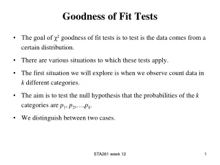
9. Tests of Goodness of Fit • The goodness-of-fit test applies only to univariate data. • The null hypothesis specifies a discrete distribution for the population. • We want to determine whether a sample from that population supports this hypothesis.

10. Examples • If we rolled a die 60 times, we expect 10 of each number. • If we get frequencies 8, 10, 14, 12, 9, 7, does that indicate that the die is not fair? • What is the distribution if the die were fair?

11. Examples • If we toss a fair coin, we should get two heads ¼ of the time, two tails ¼ of the time, and one of each ½ of the time. • Suppose we toss a coin 100 times and get two heads 16 times, two tails 36 times, and one of each 48 times. Is the coin fair?

12. Examples • If we selected 20 people from a group that was 60% male and 40% female, we would expect to get 12 males and 8 females. • If we got 15 males and 5 females, would that indicate that our selection procedure was not random (i.e., discriminatory)? • What if we selected 100 people from the group and got 75 males and 25 females?

13. Null Hypothesis • The null hypothesis specifies the probability (or proportion) for each category. • Each probability is the probability that a random observation would fall into that category.

14. Null Hypothesis • To test a die for fairness, the null hypothesis would be H0: p1 = 1/6, p2 = 1/6, …, p6 = 1/6. • The alternative hypothesis will always be a simple negation of H0: H1: At least one of the probabilities is not 1/6. or more simply, H1: H0 is false.

15. Level of Significance • Let  = 0.05. • The test statistic will involve the expected counts.

16. Expected Counts • To find the expected counts, we apply the hypothetical probabilities to the sample size. • For example, if the hypothetical probabilities are 1/6 and the sample size is 60, then the expected counts are (1/6)  60 = 10.

17. Example • The test statistic will be the 2 statistic. • Make a chart showing both the observed and expected counts (in parentheses).

18. The Chi-Square Statistic • Denote the observed counts by O and the expected counts by E. • Define the chi-square (2) statistic to be

19. The Chi-Square Statistic • Clearly, if all of the deviations O – E are small, then 2 will be small. • But if even a few the deviations O – E are large, then 2 will be large.

20. The Value of the Test Statistic • Now calculate 2.

21. Compute the p-Value • To compute the p-value of the test statistic, we need to know more about the distribution of 2.

22. Chi-Square Degrees of Freedom • The chi-square distribution has an associated degrees of freedom, just like the t distribution. • Each chi-square distribution has a slightly different shape, depending on the number of degrees of freedom. • In this test, df is one less than the number of cells.

23. Chi-Square Degrees of Freedom

24. 2(2) Chi-Square Degrees of Freedom

25. 2(2) 2(5) Chi-Square Degrees of Freedom

26. 2(2) 2(5) 2(10) Chi-Square Degrees of Freedom

27. Properties of 2 • The chi-square distribution with df degrees of freedom has the following properties. • 2  0. • It is unimodal. • It is skewed right (not symmetric!) • 2 = df. • 2 = (2df).

28. Properties of 2 • If df is large, then 2(df) is approximately normal with mean df and standard deviation (2df).

29. Chi-Square vs. Normal

30. 2(128) Chi-Square vs. Normal

31. N(128, 16) 2(128) Chi-Square vs. Normal

32. TI-83 – Chi-Square Probabilities • To find a chi-square probability (p-value) on the TI-83, • Press DISTR. • Select 2cdf (item #7). • Press ENTER. • Enter the lower endpoint, the upper endpoint, and the degrees of freedom. • Press ENTER. • The probability appears.

33. Computing the p-value • The number of degrees of freedom is 1 less than the number of categories in the table. • In this example, df = 5. • To find the p-value, use the TI-83 to calculate the probability that 2(5) would be at least as large as 3.4. • p-value = 2cdf(3.4, E99, 5) = 0.6386. • Therefore, p-value = 0.6386 (accept H0).