Download
1 / 25
260 likes | 414 Views
Standing Waves Reminder. Confined waves can interfere with their reflections Easy to see in one and two dimensions Spring and slinky Water surface Membrane For 1D waves, nodes are points For 2D waves, nodes are lines or curves. b. U = 0. U = ∞. 0. 0. a. p 2 h 2. Energies. n x.

E N D
Standing Waves Reminder • Confined waves can interfere with their reflections • Easy to see in one and two dimensions • Spring and slinky • Water surface • Membrane • For 1D waves, nodes are points • For 2D waves, nodes are lines or curves
b U = 0 U = ∞ 0 0 a p2h2 • Energies nx 2 ny 2 2m + a b Rectangular Potential • Solutions y(x,y) = A sin(nxpx/a) sin(nypy/b) • Variables separatey = X(x) · Y(y)
p2h2 • Energies nx2 + ny2 2ma2 Square Potential • Solutions y(x,y) = A sin(nxpx/a) sin(nypy/a) a U = 0 U = ∞ 0 a 0
Schrodinger Equation Uy – (h2/2M)y = Ey Combining Solutions • Wave functions giving the same E (degenerate) can combine in any linear combination to satisfy the equation A1y1 + A2y2 + ···
– + – + Square Potential • Solutions interchanging nx and ny are degenerate • Examples: nx = 1, ny = 2 vs. nx = 2, ny = 1
– + + – y1+y2 y1–y2 y2–y1 –y1–y2 – – + + + – + – Linear Combinations • y1 = sin(px/a) sin(2py/a) • y2 = sin(2px/a) sin(py/a)
y1+y2 – – + + Node at y = x y1–y2 Verify Diagonal Nodes y1 = sin(px/a) sin(2py/a) y2 = sin(2px/a) sin(py/a) Node at y = a – x
Circular membrane standing waves edge node only diameter node circular node Circular membrane • Nodes are lines Source:Dan Russel’s page • Higher frequency more nodes
Types of node • radial • angular
3D Standing Waves • Classical waves • Sound waves • Microwave ovens • Nodes are surfaces
z q r y f x Hydrogen Atom • Potential is spherically symmetrical • Variables separate in spherical polar coordinates
Quantization Conditions • Must match after complete rotation in any direction • angles q and f • Must go to zero as r ∞ • Requires three quantum numbers
We Expect • Oscillatory in classically allowed region (near nucleus) • Decays in classically forbidden region • Radial and angular nodes
Electron Orbitals • Higher energy more nodes • Exact shapes given by three quantumnumbers n,l,ml • Form ynlm(r, q, f) = Rnl(r)Ylm(q, f)
Radial Part R ynlm(r, q, f) = Rnl(r)Ylm(q, f) Three factors: • Normalizing constant (Z/aB)3/2 • Polynomial in r of degree n–1 (p. 279) • Decaying exponential e–r/aBn
Angular Part Y ynlm(r, q, f) = Rnl(r)Ylm(q, f) Three factors: • Normalizing constant • Degree l sines and cosines of q (associated Legendre functions, p.269) • Oscillating exponential eimf
Hydrogen Orbitals Source: Chem Connections “What’s in a Star?” http://chemistry.beloit.edu/Stars/pages/orbitals.html
Energies • E = –ER/n2 • Same as Bohr model
Quantum Number n • n: 1 + Number of nodes in orbital • Sets energy level • Values: 1, 2, 3, … • Higher n → more nodes → higher energy
Quantum Number l • l: angular momentum quantum number • Number of angular nodes • Values: 0, 1, …, n–1 • Sub-shell or orbital type l 0 1 2 3 orbital type s p d f
Quantum number ml • z-component of angular momentum Lz = mlh • Values: –l,…, 0, …, +l • Tells which specific orbital (2l + 1 of them) in the sub-shell l 0 1 2 3 orbital type s p d f degeneracy 1 3 5 7
Angular momentum • Total angular momentum is quantized • L = [l(l+1)]1/2h • Lz = mlh • z-component of L is quantized in increments of h • But the minimum magnitude is 0, not h
Radial Probability Density • P(r) = probability density of finding electron at distance r • |y|2dV is probability in volume dV • For spherical shell, dV = 4pr2dr • P(r) = 4pr2|R(r)|2
Radial Probability Density Radius of maximum probability • For 1s, r = aB • For 2p, r = 4aB • For 3d, r = 9aB (Consistent with Bohr orbital distances)
Quantum Number ms • Spin direction of the electron • Only two values: ± 1/2