Download
1 / 36
360 likes | 582 Views
Travel, Land Use & Smart Growth: What Don’t We Know?. Caltrans Research Connection Randy Crane, UCLA September 2004. Outline. Land Use, Smart Growth & Travel Research questions , large and small Research examples : Smart growth, VMT, and commute length Summary and next moves.

E N D
Travel, Land Use & Smart Growth:What Don’t We Know? • Caltrans Research Connection • Randy Crane, UCLA • September 2004
Outline • Land Use, Smart Growth & Travel • Research questions, large and small • Research examples: Smart growth, VMT, and commute length • Summary and next moves
Big Questions • Urban Form: Sprawl and traffic • Neighborhood Design: The influence of neighborhood features on trip taking, mode choice, physical activity,….
Big Answers • The New Urbanism: Increase densities & transit access, mix land uses more, village scale, discourage cars,.... • Smart Growth: The above + public participation and broader urban growth management strategies
Two Research Examples • Will smart growth reduce VMT? • Will smart growth shorten commutes?
Summary of Smart Growth Argument • Auto travel is increasing faster than population growth, and suburbanization, sprawl and car subsidies are to blame • In particular, more roads do not relieve congestion but transit and “smart growth” do, since both common sense and UC Berkeley studies indicate that: • Induced demand fills up roads as fast as they’re built • Higher residential densities reduce car ownership, trips/person & VMT/person • TOD and mixed land uses increase transit use, reduce parking & VMT
Bad Neighborhood vs Good Neighborhood
Problems with Early Research • Many studies indicate a lower auto mode share & VMT in higher density, mixed use areas. • But, empirical strategies for estimating and evaluating the impacts of accessibility on travel behavior were primitive. For example, • mode choice or VMT or #trips = f(density, access, pedestrian friendliness, demographics,....) • Behavioral story ad hoc; the role of conventional choice variables such as relative prices, resources, etc., unspecified.
Why a Problem? • These unresolved modeling issues, which center on the lack of a consistent behavioral framework, greatly limit the usefulness of empirical results. • For example, where are the demand elasticities, what is the performance interpretation of accessibility, how can any given set of results be transferred outside the data at hand?
Research Strategy • What we want to know: How does each neighborhood and community design feature, alone and in conjunction with others, influence travel behavior? • Consider the evidence on this question to date: Descriptive, simulation, behavioral. • A “behavioral” approach
Behavioral Model • Q: What influences travel and how do land use, density, and access reflect behavioral variables? • Model the demand for trips but make the built environment explicit. For example, say consumers make trip decisions to maximize U(a,w,x) • subject to y = x + apa + apw . The solutions to this problem are the trip demand functions a(pa,pw,y) and w(pa,pw,y). • (where a is the number of trips by automobile for each purpose, w is the number of trips by walking for each purpose, x is a composite of the time spent on other activities, pa is time per trip for travel by automobile, pw is time per trip for walking, y is the total time available for travel.)
Apply to Data • Empirical Specification: Determine how the land use measures map into the parameters (pi, mi, ti). Determine how trip purposes map into the variables (a, w). Find data corresponding to these measures. • Estimation: Specify a functional form for demand and estimate a(pa,pw,y), w(pa,pw,y), etc., as appropriate to the data.
VMT Evidence • Compact development, mixed uses, and open circulation pattern reduce length of a typical trip • But shorter trips are taken more often, so VMT could rise (or fall). • There is no clear evidence that higher densities will systematically change travel patterns beyond increasing congestion.
Mode Choice Evidence • Does compact development or transit-based housing improve ridership? Depends. • Will cities build transit-based housing? Cities see transit stations as economic development anchors and sources of labor, not as a way to get residents to work or shopping elsewhere
Completely Open questions • Trip generation of compact development vs. trip length • Impact of higher densities on total travel, mode choice, congestion, and air quality • Impact of transit-based housing or commercial development on transit ridership • Determinants of walking and biking
Smart Growth/Traffic Summary • There is no clear evidence that higher densities will systematically change travel patterns beyond increasing congestion. • Shorter trips are taken more often, VMT could rise • Cities see transit stations as economic development anchors and sources of labor, not as a way to get residents to work or shopping elsewhere • The evidence that TOD raises transit use or that the built environment influences travel behavior at the margin is weak to none
Background • 1. The CW: Increasingly, people are driving hours to work because of sprawl • 2. The evidence: Little regarding whether houses & jobs are growing farther apart -- or which industries/occupations are dispersing most • 3. Leading to the question: Since there are arguments both ways, how does the commute vary with job sprawl?
What is Sprawl? • “Smart Growth America” measures sprawl as: • One part density • One part mixed use • One part “centeredness” • One part “accessibility”
The Fort Lauderdale & Tucson areas are roughly average in the sum of these measures, with FL relatively high in access and low in centeredness, & Tucson high in mixed uses & centers. Are their traffic outcomes then similar? • (15 VMT/cap vs 20 VMT/cap)
%Population & Employment in Suburbs, 1948-1990
Commute Times in California, 1990-2000 (Census)
Basic Explanations • Monocentric model:suburban residents drive further, but are compensated by lower land rents • Basic extensions: multiple employment centers, commute patterns more complex, both rents & wages compensate
Recent Extensions • Wheaton (2002): Firms benefit from both clustering (via agglomeration economies) and from shorter commutes (via lower wages) • ➥ Shorter commutes if jobs decentralize • ➥Consistent with Gordon, Kumar, and Richardson (1989)
Crane (1996): If area polycentric, job location may change ➥Residential choice is a gamble • ➥ Rational workers will hedge bets by locating to minimize average expected commute costs • ➥ Implies longer commutes than Wheaton • ➥ Results should vary by occupation (job mobility) & life-cycle (moving costs), as in Wachs, et al. (1993)
Empirical Strategy • Specification: Explain individual commute as a function of household demand/supply factors (e.g., resources, dual earners, travel costs, tastes, etc.) • … plus regional employment deconcentration, and individual occupation and life-cycle factors • Estimation issues: Note that wages, land costs, and car access are potentially endogenous
Data • American Housing Survey: ~50,000 surveys in most metropolitan areas every two years, current sample in use since 1985. • ➥ We use only urban part for reported SMSAs • ➥ 11,000-15,000 per year, for 64,000+ total observations over 12 years • BEA county employment data by 1 digit SIC
Industry Detail Results • All these things considered, employment sprawl is associated with shorter (in distance) commutes • However, results differ by industry: • Construction & Wholesale => shorter • Manf & Govt. => longer • Retail & Service => same
Commuting Conclusions • No definitive answers. Some support for argument that both firms & workers value shorter commutes & locate accordingly, but results differ by industry • ➥ Need better detail on employment sprawl • Less support for argument that job mobility, with life-cycle effects, lengthens commutes • ➥ Need data on occupation & moving costs
Overall Summary • Urban Form and Land Use certainly influence transportation behavior, but we do not have confidence about the details • Smart Growth is a sincere, hopeful effort to provide more consistent and participatory planning, but its specific transportation claims are mainly speculative • Better data and better empirical methods in understanding the interaction of urban design & transportation are on the way. In the meantime, a case by case approach is advised.