Conclusions

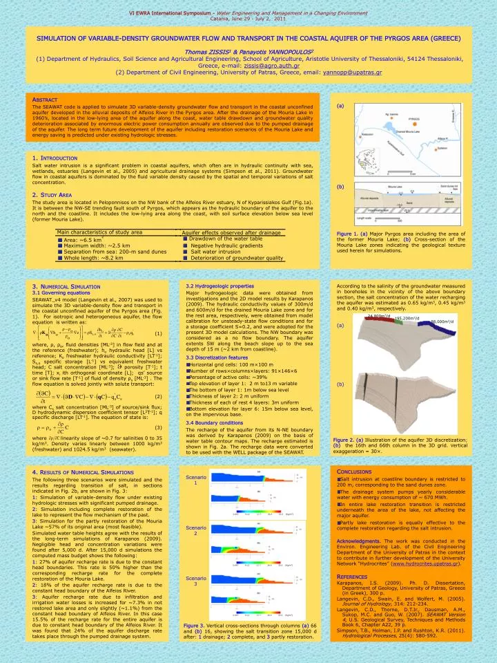
1. VI EWRA International Symposium - Water Engineering and Management in a Changing Environment Catania, June 29 - July 2, 2011 Abstract • The SEAWAT code is applied to simulate 3D variable-density groundwater flow and transport in the coastal unconfined aquifer developed in the alluvial deposits of Alfeios River in the Pyrgos area. After the drainage of the Mouria Lake in 1960’s, located in the low-lying area of the aquifer along the coast, water table drawdown and groundwater quality deterioration associated by enormous electric power consumption annually are observed due to the pumped drainage of the aquifer. The long term future development of the aquifer including restoration scenarios of the Mouria Lake and energy saving is predicted under existing hydrologic stresses. Introduction Salt water intrusion is a significant problem in coastal aquifers, which often are in hydraulic continuity with sea, wetlands, estuaries (Langevin et al., 2005) and agricultural drainage systems (Simpson et al., 2011). Groundwater flow in coastal aquifers is dominated by the fluid variable density caused by the spatial and temporal variations of salt concentration. Study Area The study area is located in Peloponnisos on the NW bank of the Alfeios River estuary, N of Kyparissiakos Gulf (Fig.1a). It is between the NW-SE trending fault south of Pyrgos, which appears as the hydraulic boundary of the aquifer to the north and the coastline. It includes the low-lying area along the coast, with soil surface elevation below sea level (former Mouria Lake). SIMULATION OF VARIABLE-DENSITY GROUNDWATER FLOW AND TRANSPORT IN THE COASTAL AQUIFER OF THE PYRGOS AREA (GREECE)Thomas ZISSIS1 & Panayotis YANNOPOULOS2 (1) Department of Hydraulics, Soil Science and Agricultural Engineering, School of Agriculture, Aristotle University of Thessaloniki, 54124 Thessaloniki, Greece, e-mail: zissis@agro.auth.gr(2) Department of Civil Engineering, University of Patras, Greece, email: yannopp@upatras.gr Numerical Simulation 3.1 Governing equations SEAWAT_v4 model (Langevin et al., 2007) was used to simulate the 3D variable-density flow and transport in the coastal unconfined aquifer of the Pyrgos area (Fig. 1). For isotropic and heterogeneous aquifer, the flow equation is written as: (1) where, ρ, ρο, fluid densities [ML-3] in flow field and at the reference (freshwater); ho hydraulic head [L] vs reference; Ko freshwater hydraulic conductivity [LT-1]; Ss,o specific storage [L-1] vs equivalent freshwater head; C salt concentration [ML-3]; porosity [T-1]; t time [T]; xiith orthogonal coordinate [L]; qs’ source or sink flow rate [T-1] of fluid of density ρs [ML-3] . The flow equation is solved jointly with solute transport: (2) where Cs salt concentration [ML-3] of source/sink flux; D hydrodynamic dispersion coefficient tensor [L2T-1]; q specific discharge [LT-1]. The equation of state is: (3) where linearity slope of ~0.7 for salinities 0 to 35 kg/m3. Density varies linearly between 1000 kg/m3 (freshwater) and 1024.5 kg/m3 (seawater). 3.2 Hydrogeologic properties Major hydrogeologic data were obtained from investigations and the 2D model results by Karapanos (2009). The hydraulic conductivity values of 300m/d and 600m/d for the drained Mouria Lake zone and for the rest area, respectively, were obtained from model calibration for unsteady-state flow conditions and for a storage coefficient S=0.2, and were adopted for the present 3D model calculations. The NW boundary was considered as a no flow boundary. The aquifer extents SW along the beach slope up to the sea depth of 15 m (~2 km from coastline). 3.3 Discretization features Horizontal grid cells: 100 m×100 m Number of rows×columns×layers: 91×146×6 Persentage of active cells: ~39% Top elevation of layer 1: 2 m to13 m variable The bottom of layer 1: 1m below sea level Thickness of layer 2: 2 m uniform Thickness of each of rest 4 layers: 3m uniform Bottom elevation for layer 6: 15m below sea level, on the impervious base. 3.4 Boundary conditions The recharge of the aquifer from its N-NE boundary was derived by Karapanos (2009) on the basis of water table contour maps. The recharge estimated is shown in Fig. 2a. The recharge data were converted to be used with the WELL package of the SEAWAT. According to the salinity of the groundwater measured in boreholes in the vicinity of the above boundary section, the salt concentration of the water recharging the aquifer was estimated as 0.65 kg/m3, 0.45 kg/m3 and 0.40 kg/m3, respectively. (a) (b) (a) (b) Figure 1. (a) Major Pyrgos area including the area of the former Mouria Lake; (b)Cross-section of the Mouria Lake zones indicating the geological texture used herein for simulations. Figure 2. (a) Illustration of the aquifer 3D discretization; (b) the 16th and 66th column in the 3D grid. Vertical exaggeration = 30×. • 4. Results of Numerical Simulations • The following three scenarios were simulated and the results regarding transition of salt, in sections indicated in Fig. 2b, are shown in Fig. 3: • 1: Simulation of variable-density flow under existing hydrologic stresses with significant pumped drainage. • 2: Simulation including complete restoration of the lake to represent the flow mechanism of the past. • 3: Simulation for the partly restoration of the Mouria Lake ~57% of its original area (most feasible). • Simulated water table heights agree with the results of the long-term simulations of Karapanos (2009). Negligible head and concentration variations were found after 5,000 d. After 15,000 d simulations the computed mass budget shows the following: • 1: 27% of aquifer recharge rate is due to the constant head boundaries. This rate is 50% higher than the corresponding recharge rate for the complete restoration of the Mouria Lake. • 2: 18% of the aquifer recharge rate is due to the constant head boundary of the Alfeios River. • 3: Aquifer recharge rate due to infiltration and irrigation water losses is increased for ~7.3% in not restored lake area and only slightly (~1.1%) from the constant head boundary of Alfeios River. In this case 15.5% of the recharge rate for the entire aquifer is due to constant head boundary of the Alfeios River. It was found that 24% of the aquifer discharge rate takes place through the pumped drainage system. Scenario 1 Scenario 2 Scenario 3 • Conclusions • Salt intrusion at coastline boundary is restricted to 200 m, corresponding to the sand dunes zone. • The drainage system pumps yearly considerable water with energy consumption of ~ 670 MWh. • In entire lake restoration transition is restricted underneath the area of the lake, not affecting the major aquifer. • Partly lake restoration is equally effective to the complete restoration regarding the salt intrusion. • Acknowledgments.The work was conducted in the Environ. Engineering Lab. of the Civil Engineering Department of the University of Patras in the context to contribute in further development of the University Network “Hydrocrites” (www.hydrocrites.upatras.gr). • References • Karapanos, I.S. (2009). Ph. D. Dissertation, Department of Geology, University of Patras, Greece (in Greek), 300 p. • Langevin, C.D., Swain, E. and Wolfert, M. (2005). Journal of Hydrology, 314: 212-234. • Langevin, C.D., Thorne, D.T.Jr., Dausman, A.M., Sukop, M.C. and Guo, W. (2007). SEAWAT Version 4, U.S. Geological Survey, Techniques and Methods Book 6, Chapter A22, 39 p. • Simpson, T.B., Holman, I.P. and Rushton, K.R. (2011). Hydrological Processes, 25(4): 580-592. 24,800m3/d 195,200m3/d 88,000m3/d Figure 3.Vertical cross-sections through columns (a) 66 and (b) 16, showing the salt transition zone 15,000 d after: 1 drainage; 2 complete, and 3 partly restoration.