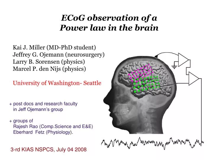
ECoG observation of a Power law in the brain

1. ECoG observation of a Power law in the brain Kai J. Miller (MD-PhD student) Jeffrey G. Ojemann (neurosurgery) Larry B. Sorensen (physics) Marcel P. den Nijs (physics) University of Washington- Seattle + post docs and research faculty in Jeff Ojemann’s group + groups of Rajesh Rao (Comp.Science and E&E) Eberhard Fetz (Physiology). 3-rd KIAS NSPCS, July 04 2008

2. Outline • General Introduction • Review of basic brain physiology • Earlier power law tries. • Our experiment set-up and issues • Power law analysis • Conclusions

3. EEG (electroencephalograph) rhythms Richard Caton (1875) - animals Berger (1924) -humans Brain computer interface (machine learning); play video games without hands or control robotic arms. power freq

4. Available Experimental probes: • EEG (electroencephalography) • (electrodes (ohmic) on skull, low resolution, weak electric signal). • ECoG (electrocorticography) • (electrodes directly on the cortex, high spatial and temporal • resolution, portable, invasive). • MRI (magnetic resonance imaging) • (couples to blood flow (local metabolism), non-invasive, low • temporal and spatial resolution). • MEG (magnetoencephalography) • (couples to magnetic field generated by electric currents, • non-invasive, good resolution, inversion problem, not portable).

5. Electrocorticographic (ECoG) Arrays • Electrodes placed directly on the cortex • Placed for 4-7 days in context of seizure focus localization during epilepsy treatment • Platinum electrodes • 4 mm in diameter • 2.3 mm exposed • Separated by 1cm center-to-center • 8x8 arrays and/or linear strips

6. Electrocorticographic (ECoG) Arrays • Electrodes placed directly on the cortex • Placed for 4-7 days in context of seizure focus localization during epilepsy treatment • Platinum electrodes • 4 mm in diameter • 2.3 mm exposed • Separated by 1cm center-to-center • 8x8 arrays and/or linear strips

7. Electrocorticographic (ECoG) Arrays • In this study array located in the motor area of cortex. • Sampled at 10kHz or 1KHz or 2 KHz • Fixation task: subject fixates on a “x” on wall 3m from hospital bed for 130-190 seconds. • Nearest neighbor electrode pair wise referencing. • Fourier transform V(t) 1 sec long sets (Hann windowed). • Power spectra P(f) averaged over sets.

8. Shift in cortical power spectrum with simple movement repetition Kai+ Jeff main discovery: LOW FREQUENCY DECREASE in power (inhibitory) HIGH FREQUENCY INCREASE with activity Kai Miller et.al., 2007, J Neuroscience

9. Shift in cortical power spectrum with simple movement repetition AND: At frequencies larger than 40 Hz the power spectrum is not dominated by sharp peaks (rhythms) anymore. It is a broad band ---> does it follow a power law shape?

10. Goals and Issues: • clinical: Brain surgery is local. ECoG is a local probe. • The high frequency (f>70 Hz) up-shift with activity represents local • phenomena (e.g., in finger/thumb motor area) while the EEG low • frequency rhythms likely represent more global control features. • Need to map out areas of specific local functionality and correlations • between those areas. • engineering: build computer brain interfaces (machine learning, robotic • arms, cell-phone implants….. brave new world). • fundamental research: How do our brains compute? • How fast do they compute? • How do they store/retrieve information? • How universal is all of the above? • Can we do quantitative neuroscience/biophysics? • Let’s test this on the power spectrum: • -- How well can we confirm/disprove a power law form at f>70Hz? • -- Does universality hold/apply (robust power law exponent)?

11. from 80 - 500Hz At high frequencies, the averaged power spectrum obeys a power law

12. Outline • General Introduction • Review of basic brain physiology • Earlier power law tries. • Our experiment set-up and issues • Power law analysis • Conclusions

13. Large scale organization of the Cortex: Brodmann area’s (http://www.umich.edu/~cogneuro/jpg/Brodmann.html)

14. The cortex is a thin sheet about 0.5 m wide and 2-3 mm thick, folded inside the skull. gray matter: neurons white matter: cables (axons) underneath each ECoG electrode: about 106 neurons each with up to 104 synapses. (figures from Nunez-1981-2005, Hamalainen RMP1993)

15. computations within a neuron -> axon pulses arrive at (several) synapses -> neurotransmitters diffuse across gaps -> post synaptic potential -> dendritic tree computation (integration; more?) -> axon fires pulse if potential above threshold Total time scale= 5-10 msec Until recently dendrites were believed to be passive. That would have implied: linear cable theory -> superposition principle -> simple integrator of excitatory & inhibitory synapse connections. Dendritic tree computations might act like preprogrammed “subroutines” that “code associations” Synaptic plasticity acts within minutes

16. from Koch “Biophysics of Computation”

17. Ion pumps create local electric current sources Ion pumps at synapses induce electric charge currents along dendrites; represent dipole current fields; they are collectively aligned. Charge neutral character of axon soliton-shaped pulses implies no macroscopic charge transport; creates only local quadrupole and higher order type current fields.

18. EEG and ECoG measure electric dipole current fields created by: synaptic, dendritic, axon charge/spike currents and associated chemical transmitters and ion channel currents; propagated in a messy ionic solution environment (membranes, glial cells,…). Think of: electrodes attached to a saltwater bath where this ``battery” contains very many small active pumps stirring-up internal electric dipole currents. (Synaptic ones dominate.) Power spectrum measures the Fourier transform of the auto-correlation function

19. Electric current dipole fields: (see: Nunez-1981-2005, Hamalainen RMP1993)

20. Time scales: • typical reaction time to external inputs (“move index finger”) is ~ 1sec. • basic processes in brain/neural system take about 10 msec: • -- spike speed in axon 1-10m/sec (myelin cover layer); • -- synaptic connection (neurotransmitter diffusion): ~10 msec • -- computation within dendritic tree: a few ms • so, only ~100 steps available -> massive “parallel” computations (synchronization) • Scale free network? • Memory retrieval is fast compared to 10 msec time scale. • How can it not use a scale free network topology for that • (or do something better)? • Scale free avalanche behavior? • Some in vitro (rat brain culture) data and some simple modeling • Time correlations between spikes (in one neuron and more globally between • neurons is to be expected. • Might expect therefore power laws in power spectrum; • but almost everything is still open to discussion/interpretation in this very • complex functional and many component system.

21. Outline • General Introduction • Review of basic brain physiology • Earlier power law tries. • Our experiment set-up and issues • Power law analysis • Conclusions

22. Earlier power law fits (EEG)

23. Our results: quantitative high accuracy scaling over 4 decades in power (vertical axis) between 80 Hz<f<400H Global power spectrum (excluding the EEG low freq rhythms) obeys the form L + L =4.0(1) f0=70(5) Hz L=2.0(4)

24. Outline • General Introduction • Review of basic brain physiology • Earlier power law tries. • Our experiment set-up and issues • Power law analysis • Conclusions

25. Each channel voltage is referenced with respect to a common reference electrode somewhere on the skull. We referenced them as nearest neighbor electrode pairs. This takes out common far away sources. The signal from electrode pars varies a lot; due to variations In quality of electrode-pia-cortex contact and the presence of nearby blood vessels. The most obvious very weak ones can be removed from ensemble.

26. Power spectrum handling & auto correlation function

27. Gain-corrected Raw Gain and Floor Corrected Spectrum Amplifier low pass filter (roll-off) and noise floors issues: Noise Floor Amplitude Gain Frequency Response

28. Amplifier low-pass filtering (roll-off) Measured independently at this 10kHz sampling rate settings.

29. Gain-corrected Raw Gain and Floor Corrected Spectrum Noise Floor Amplitude Gain Frequency Response

30. Noise floor originates from the amplifiers. We treated the noise floor as a ``fitting parameter”. We also measured the floors independently “in-situ” without cortex but electrode array and clinical amplifiers in place. Results have correct magnitude; but are suspected to vary in time (days) between subjects. The noise floors are high as amplifiers go, but no alternative available (yet) because they need to be FDA approved.

31. Gain-corrected Raw Gain and Floor Corrected Spectrum Noise Floor Amplitude Gain Frequency Response

32. Outline • General Introduction • Review of basic brain physiology • Earlier power law tries. • Our experiment set-up and issues • Power law analysis • Conclusions

33. from 80 - 500Hz At high frequencies, the averaged power spectrum obeys a power law

34. Channel pair averaged power spectrum Subject 1 illustration noise floor fitting range: above: below 250 Hz the fit is insensitive to the noise floor (C=13000 shown) right: C= 15500 fits data globally until 500~Hz

35. Fitted noise floor, C=15700 (S1), somewhat higher than average signal at higher frequencies; but near signal noise limit; maybe amplifier noise not truly white, or varies somewhat with input, or …… ……….. Need better amplifiers…..

36. Range shrinking fitting protocol

37. Universality in area underneath the electrode array. Width of histogram of power law exponents is consistent with systematic issues (e.g., nearby blood vessels reduce the signal-> hit amplifier noise floor earlier, reduced accuracy). Universality? Yes within and across subjects S1 and S2.

38. Knee!!! Global power spectrum structure.  for f>70 Hz Crossover at f=70 Hz visible in S1; obscured in S2.  and  rhythms very small in 8 channel pairs of S1; prominent in all channel pairs of S2. Simple minded linear log-log fit for 15-80Hz in 8 channel pairs of S1 yield L=2.57 (std 0.15). But this data set quite small …..

39. “Global” power spectrum and corrections to scaling Those local fits may look good, but it is the wrong type of fit; need to take into account corrections to scaling from f>70Hz region. with as condition L + L =4 and f0=70Hz yields L=2.0 (std 0.4) withfL<1Hz for S1 and also in 1kHz data sets

40. Low frequency fits from (older) 1kHz data sets with small  rhythm peaks • 16 Subjects: Basic fixation on an “x” on the hospital room wall, 3-4 meters away 2-3 min. • 1 kHz sample rate. • Pair wise difference re-referencing between electrodes (32 electrodes, 52 channel pairs). • Power Spectral Density calculated using FFT of overlapping Hann Windows (1 sec in length). • Each spectrum corrected for amplifier roll-off (but not for noise floor) • “Unbiased” selection of 116 channel pairs that lack prominent rhythms.

41. 1 kHz fixation data fit from 15-80Hz Simple fits yield (again) = 2.5 (STD=0.4, N=116) Crosover scaling 2-powers fit, with L + H =4 as constraint yields (again) = 2.0 (STD=0.4, N=116)

42. In general, with specific tasks like hand or tongue movement, we need to decompose the EEG rhythms from the broadband to test for universality Is the same power law present underneath the  rhythms (universality)?

43. Separation hypothesis has been achieved qualitatively already with a principal component analysis Miller et.al., 2007, J. Neuroscience rhythm peaks power law: P(f) ~ freq - superposition actual data (at 1kHz sampling)

44. Outline • General Introduction • Review of basic brain physiology • Earlier power law tries. • Our experiment set-up and issues • Power law analysis • Conclusions

45. Interpretation of the powerlaw ? If L and/or  had been not integer, we would have been safe to argue to have seen scale free complex brain behavior. Still possible with current error bar in L=2.0 (0.4), but…. it could well be the product of two simple Lorentzians L=H=2 Those can arise in many contexts: Low pass filters, form factors (spike and/or avalanche shapes), exponential decaying auto-correlation correlation functions….. Too many options to decide at this point… Needs further theory-experiment interactions to weed out possibilities!

46. Summary

47. Summary

48. Summary

49. Summary

50. Summary