Download
1 / 41
410 likes | 514 Views
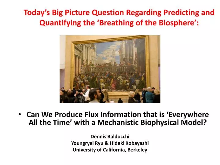
Today’s Big Picture Question Regarding Predicting and Quantifying the ‘Breathing of the Biosphere’:. Can We Produce Flux Information that is ‘Everywhere All the Time’ with a Mechanistic Biophysical Model?. Dennis Baldocchi Youngryel Ryu & Hideki Kobayashi University of California, Berkeley.

E N D
Today’s Big Picture Question Regarding Predicting and Quantifying the ‘Breathing of the Biosphere’: • Can We Produce Flux Information that is ‘Everywhere All the Time’ with a Mechanistic Biophysical Model? Dennis Baldocchi YoungryelRyu & Hideki Kobayashi University of California, Berkeley
How Do We Transcend Flux Information from the Scales of the Stomata to the Leaf, Plant, Lanscape and Globe? Globe: 10,000 km (107 m) Continent: 1000 km (106 m) Landscape: 1-100 km Canopy: 100-1000 m Plant: 1-10 m Leaf: 0.01-0.1 m Stomata: 10-5m Bacteria/Chloroplast: 10-6 m
A Challenge for Leaf to Landscape Upscaling: Transform Weather Conditions from a Weather Station to that of the Leaves in a Canopy with Their Assortment of Angles and Layers Relative to the Sun and Sky And use that information to drive a variety of Non-Linear Functions (photosynthesis, energy balance, stomatal conductance)
The Perils of Upscaling Leaf-Scale Fluxes ‘.. To build a model we have to consider and join two levels of knowledge. The level with the sort of relaxation times is then the level which provides the explanation or the explanatory level and the one with the long relaxation times, the level which is to be explained or the explainable level…’ Cornelus T deWit (1970)
Upscaling from Landscapes to the Globe ‘Space: The final frontier … To boldly go where no man has gone before’ Captain James Kirk, Starship Enterprise
Global-Scale SVAT Modeling is Possible Today Piers Sellers, Biometeorologist(and Astronaut), broke the ‘deWit’ barrier by attempting to incorporate Soil-Vegetation-Atmosphere Transfer models (SVATS) into Global Circulation Climate Models, but at coarse spatial resolution
Challenge for Landscape to Global Upscaling Converting Virtual ‘Cubism’ back to Virtual ‘Reality’ Realistic Spatialization of Flux Data Requires the Merging Numerous Data Layers with varying Time Stamps (hourly, daily, weekly), Spatial Resolution (1 km to 0.5 degree) and Data Sources (Satellites, Flux Networks, Climate Stations)
To Develop a Scientifically Defensible Virtual World‘You Must get your boots dirty’, tooCollecting Real Data Gives you Insights on What is Important & Data to Parameterize and Validate Models
Motivation for a High-Resolution, Space-Driven, and Mechanistic Trace Gas Exchange Model • Current Global-Scale Remote Sensing Products tend to rely on • Highly-Tuned Light Use Efficiency Approach • GPP=PAR*fPAR*LUE (since Monteith 1960’s) • Empirical, Data-Driven Approach (machine learning technique) • Some Forcings come from Satellite Remote Sensing Snap Shots, at fine Spatial scale ( < 1 km) • Other Forcings come from coarse reanalysis data (several tens to hundreds of km resolution) • Hypothesis, We can do Better by: • Applying the Principles taught in Biometeorology 129 and Ecosystem Ecology 111 which Reflect Intellectual Advances in these Fields over the past Decade and Emerging Scaling Rules • Merging Vast Environmental Databases at same resolution • Utilizing Microsoft Cloud Computational Resources
Lessons Learned from the John Norman, Experience with the CanOakModel, and Reading the Literature We Must: • Couple Carbon and Water Fluxes • Assess Non-Linear Biophysical Functions with Leaf-Level Microclimate Conditions • Consider Sun and Shade fractions separately • Consider effects of Clumped Vegetation on Light Transfer • Consider Seasonal Variations in Physiological Capacity of Leaves and Structure of the Canopy
BESS, Breathing-Earth Science Simulator Atmospheric radiative transfer Beam PAR NIR Diffuse PAR NIR Rnet shade sunlit LAI, Clumping-> canopy radiative transfer Canopy photosynthesis, Evaporation, Radiative transfer Albdeo->Nitrogen -> Vcmax, Jmax Surface conductance dePury & Farquhar two leaf Photosynthesis model Penman-Monteith evaporation model Radiation at understory Soil evaporation Soil evaporation
Necessary Attributes of Global Biophysical ET Model: Applying Lessons from the Berkeley Biomet Class and CANOAK • Treat Canopy as Dual Source (Sun/Shade), Two-Layer (Vegetation/Soil) system • Treat Non-Linear Processes with Statistical Rigor (Norman, 1980s) • Requires Information on Direct and Diffuse Portions of Sunlight • Monte Carlo Atmospheric Radiative Transfer model (Kobayashi + Iwabuchi,, 2008) • Couple Carbon-Water Fluxes for Constrained Stomatal Conductance Simulations • Photosynthesis and Transpiration on Sun/Shade Leaf Fractions (dePury and Farquhar, 1996) • Compute Leaf Energy Balance to compute Leaf Saturation Vapor Pressure and Respiration Correctly • Photosynthesis of C3 and C4 vegetation Must be considered Separately • Light transfer through canopies MUST consider Leaf Clumping to Compute Photosynthesis/Stomatal Conductance correctly (Baldocchi and Harley, 1995) • Apply New Global Clumping Maps of Chen et al./Pisek et al. • Use Emerging Ecosystem Scaling Rules to parameterize models, based on remote sensing spatio-temporal inputs • Vcmax=f(N)=f(albedo) (Ollinger et al; Hollinger et al; Wright et al.) • Seasonality in Vcmax is considered (Wang et al., 2008) • Vcmax scales with Jmax (Wullschleger, 1993 )
Youngryel was lonely with 1 PC Challenge for a Computationally-Challenged Biometeorology Lab: Extracting Data Drivers from Global Remote Sensing to Run the Model Atmospheric radiative transfer MOD04 aerosol MOD05 Precipitable water Net radiation MOD06 cloud MOD07 Temperature, ozone MCD43 albedo MOD11 Skin temperature MOD15 LAI Canopy radiative transfer POLDER Foliage clumping
Barriers to Global Remote Sensing by the Berkeley Biometeorology Lab • Data processing • Global 1-year source data: 2.4 TB (10 yr: 24 TB) • 150,000+ source files • Global 1-year calculation: 9000 CPU hours • That is, 375 days. • 1-year calculation takes 1 year!
Help from ModisAzure -Azure Service for Remote Sensing Geoscience Source Imagery Download Sites • Scientists Scientific Results Download Request Queue . . . Download Queue Source Metadata Data Collection Stage AzureMODIS Service Web Role Portal • Science results Reprojection Queue ReprojectionStage Derivation ReductionStage Analysis Reduction Stage Reduction #1 Queue Reduction #2 Queue • AZURE Cloud with 200 CPUs cuts 1 Year of Processing to <2 days
Photosynthetic Capacity Leaf Area Index Solar Radiation Humidity Deficits
BESS vs Machine Learning Upscaling Method Ryu et al (Accepted) Global Biogeochemical Cycles
Global Evaporation at 1 to 5 km scale <ET> = 503 mm/y == 6.5 1013 m3/y An Independent, Bottom-Up Alternative to Residuals based on the Global Water Balance, ET = Precipitation - Runoff
BESS vs Machine Learning Upscaling Method Ryu et al (Accepted) Global Biogeochemical Cycles
Big Picture Question Regarding Predicting and Quantifying the ‘Breathing of the Biosphere’: • Can We Produce Flux Information with a Mechanistic Model that is ‘Everywhere, All the Time?’...Yes
Gross Photosynthesis, GPP, Across the US Lessons for Biofuel Production Indicates Less GPP in the Corn Belt, than the Adjacent Temperate Forests
Key point: 4. Temporal upscaling of fluxes from snap-shots to 8-day mean daily sum estimates Satellite overpass time 30 min Rg at TOA Day (1-8) Instantaneous LE RgPOT =f(latitude, longitude, time) Ryu et al (2011) Agricultural and Forest Meteorology Accepted
Tested the scheme using 33 flux tower data from the Arctic to the Tropics Ryu et al (Accepted) Agricultural and Forest Meteorology
Conclusion • Three-Dimensional Radiative Transfer models should be used to compute Mass and energy exchanges of Heterogeneous canopies • Models can be implemented with new generation of LIDAR data and powerful clusters of computers • Advances in Theory, Data Availability, Data Sharing and Computational Systems Enable us to Produce the Next-Generation of Globally-Integrated Products on the ‘Breathing of the Earth’ • Data-Mining these Products has Much Potential for Regional and Locale Decision making on Environmental and Agricultural Management
Data standardization MODIS Land products: standardized tiles (sinusoidal projection)
Barriers for global RS study • 2. Data standardization MODIS Atmospheric products: swath => Should be gridded to overlay with the land products
Current status • The Cloud includes • 10-year MODIS Terra and Aqua data over the US (1 km resolution) • 3-year MODIS Terra for the global land (5 km resolution) • Quota: • 200 CPUs • 100TB storage
Necessary Attributes of the Next-Generation Global Biophysical Model, BESS • Direct and Diffuse Sunlight • Monte Carlo Atmospheric Radiative Transfer model (Kobayashi, xxxx) • Light transfer through canopies consider leaf clumping • Coupled Carbon-Water for Better Stomatal Conductance Simlulations • Photosynthesis and Transpiration on Sun/Shade Leaf Fractions (dePury and Farquhar, 1996) • Photosynthesis of C3 and C4 vegetation considered • Ecosystem Scaling Relations to parameterize models, based on remote sensing spatio-temporal inputs • Vcmax=f(N)=f(albedo) (Ollinger et al; Hollinger et al;Schulze et al.; Wright et al. • Seasonality in Vcmax is considered • Model Predictions should Match Fluxes Measured at Ecosystem Scale hourly and seasonally.
Seasonal pattern of Vmax@25 follows the seasonal pattern of LAI (modified version of Houborg et al 2009 AFM)
Size and Number of Candidate Data Sets is Enormous US: 15 tiles FluxTower: 32 tiles Global: 193 tiles • Global 1-year source data: 2.4 TB (10 yr: 24 TB) • How to know which source files are missed • among >0.1 million files
Tasked Performed with MODIS-AZURE • Automation • Downloads thousands of files of MODIS data from NASA ftp • Reprojection • Converts one geo-spatial representation to another. • Example: latitude-longitude swaths converted to sinusoidal cells to merge MODIS Land and Atmosphere Products • Spatial resampling • Converts one spatial resolution to another. • Example is converting from 1 km to 5 km pixels. • Temporal resampling • Converts one temporal resolution to another. • Converts daily observation to 8 day averages. • Gap filling • Assigns values to pixels without data either due to inherent data issues such as clouds or missing pixels. • Masking • Eliminates uninteresting or unneeded pixels. • Examples are eliminating pixels over the ocean when computing a land product or outside a spatial feature such as a watershed. h08v04 h09v04 h10v04 h11v04 h12v04 h13v04 Reprojected Data (Sinusoidal format - equal land area pixel) h08v05 h09v05 h10v05 h11v05 h12v05 h08v06 h09v06 h10v06 h11v06
Components of an Integrated Earth System EXIST, but are Multi-Faceted forestinventoryplot century Forest/soil inventories decade Landsurface remote sensing Eddycovariancetowers talltowerobser- vatories remote sensingof CO2 year Temporal scale month week day hour local 0.1 1 10 100 1000 10 000 global Countries plot/site EU Spatial scale [km] From: Markus Reichstein, MPI
Computing Carbon Dioxide and Water Vapor Fluxes Everywhere, All of the Time Dennis Baldocchi Youngryel Ryu & Hideki Kobayashi University of California, Berkeley AGU, Fall 2011