Evolutionary Computing

1. Dr. T presents… Evolutionary Computing Computer Science 348

2. Introduction • The field of Evolutionary Computing studies the theory and application of Evolutionary Algorithms. • Evolutionary Algorithms can be described as a class of stochastic, population-based local search algorithms inspired by neo-Darwinian Evolution Theory.

3. Computational Basis • Trial-and-error (aka Generate-and-test) • Graduated solution quality • Stochastic local search of solution landscape

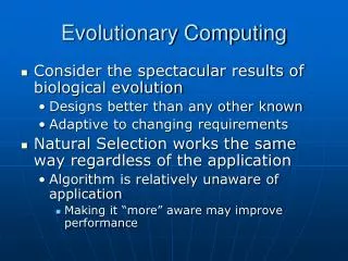
4. Biological Metaphors • Darwinian Evolution • Macroscopic view of evolution • Natural selection • Survival of the fittest • Random variation

5. Biological Metaphors • (Mendelian) Genetics • Genotype (functional unit of inheritance) • Genotypes vs. phenotypes • Pleitropy: one gene affects multiple phenotypic traits • Polygeny: one phenotypic trait is affected by multiple genes • Chromosomes (haploid vs. diploid) • Loci and alleles

6. EA Pros • More general purpose than traditional optimization algorithms; i.e., less problem specific knowledge required • Ability to solve “difficult” problems • Solution availability • Robustness • Inherent parallelism

7. EA Cons • Fitness function and genetic operators often not obvious • Premature convergence • Computationally intensive • Difficult parameter optimization

8. EA components • Search spaces: representation & size • Evaluation of trial solutions: fitness function • Exploration versus exploitation • Selective pressure rate • Premature convergence

9. Nature versus the digital realm

10. EA Strategy Parameters • Population size • Initialization related parameters • Selection related parameters • Number of offspring • Recombination chance • Mutation chance • Mutation rate • Termination related parameters

11. Problem solving steps • Collect problem knowledge • Choose gene representation • Design fitness function • Creation of initial population • Parent selection • Decide on genetic operators • Competition / survival • Choose termination condition • Find good parameter values

12. Function optimization problem Given the function f(x,y) = x2y + 5xy – 3xy2 for what integer values of x and y is f(x,y) minimal?

13. Function optimization problem Solution space: ZxZ Trial solution: (x,y) Gene representation: integer Gene initialization: random Fitness function: -f(x,y) Population size: 4 Number of offspring: 2 Parent selection: exponential

14. Function optimization problem Genetic operators: • 1-point crossover • Mutation (-1,0,1) Competition: remove the two individuals with the lowest fitness value

16. Measuring performance • Case 1: goal unknown or never reached • Solution quality: global average/best population fitness • Case 2: goal known and sometimes reached • Optimal solution reached percentage • Case 3: goal known and always reached • Convergence speed

17. Initialization • Uniform random • Heuristic based • Knowledge based • Genotypes from previous runs • Seeding

18. Representation (§2.3.1) • Genotype space • Phenotype space • Encoding & Decoding • Knapsack Problem (§2.4.2) • Surjective, injective, and bijective decoder functions

19. Simple Genetic Algorithm (SGA) • Representation: Bit-strings • Recombination: 1-Point Crossover • Mutation: Bit Flip • Parent Selection: Fitness Proportional • Survival Selection: Generational

20. Trace example errata • Page 39, line 5, 729 -> 784 • Table 3.4, x Value, 26 -> 28, 18 -> 20 • Table 3.4, Fitness: • 676 -> 784 • 324 -> 400 • 2354 -> 2538 • 588.5 -> 634.5 • 729 -> 784

21. Representations • Bit Strings • Scaling Hamming Cliffs • Binary vs. Gray coding (Appendix A) • Integers • Ordinal vs. cardinal attributes • Permutations • Absolute order vs. adjacency • Real-Valued, etc. • Homogeneous vs. heterogeneous

22. Permutation Representation • Order based (e.g., job shop scheduling) • Adjacency based (e.g., TSP) • Problem space: [A,B,C,D] • Permutation: [3,1,2,4] • Mapping 1: [C,A,B,D] • Mapping 2: [B,C,A,D]

23. Mutation vs. Recombination • Mutation = Stochastic unary variation operator • Recombination = Stochastic multi-ary variation operator

24. Mutation • Bit-String Representation: • Bit-Flip • E[#flips] = L * pm • Integer Representation: • Random Reset (cardinal attributes) • Creep Mutation (ordinal attributes)

25. Mutation cont. • Floating-Point • Uniform • Nonuniform from fixed distribution • Gaussian, Cauche, Levy, etc. • Permutation • Swap • Insert • Scramble • Inversion

26. Permutation Mutation • Swap Mutation • Insert Mutation • Scramble Mutation • Inversion Mutation (good for adjacency based problems)

27. Recombination • Recombination rate: asexual vs. sexual • N-Point Crossover (positional bias) • Uniform Crossover (distributional bias) • Discrete recombination (no new alleles) • (Uniform) arithmetic recombination • Simple recombination • Single arithmetic recombination • Whole arithmetic recombination

28. Recombination (cont.) • Adjacency-based permutation • Partially Mapped Crossover (PMX) • Edge Crossover • Order-based permutation • Order Crossover • Cycle Crossover

29. Permutation Recombination Adjacency based problems • Partially Mapped Crossover (PMX) • Edge Crossover Order based problems • Order Crossover • Cycle Crossover

30. PMX • Choose 2 random crossover points & copy mid-segment from p1 to offspring • Look for elements in mid-segment of p2 that were not copied • For each of these (i), look in offspring to see what copied in its place (j) • Place i into position occupied by j in p2 • If place occupied by j in p2 already filled in offspring by k, put i in position occupied by k in p2 • Rest of offspring filled by copying p2

31. Order Crossover • Choose 2 random crossover points & copy mid-segment from p1 to offspring • Starting from 2nd crossover point in p2, copy unused numbers into offspring in the order they appear in p2, wrapping around at end of list

32. Population Models • Two historical models • Generational Model • Steady State Model • Generational Gap • General model • Population size • Mating pool size • Offspring pool size

33. Parent selection • Fitness Proportional Selection (FPS) • High risk of premature convergence • Uneven selective pressure • Fitness function not transposition invariant • Windowing, Sigma Scaling • Rank-Based Selection • Mapping function (ala SA cooling schedule) • Linear ranking vs. exponential ranking

34. Sampling methods • Roulette Wheel • Stochastic Universal Sampling (SUS)

35. Rank based sampling methods • Tournament Selection • Tournament Size

36. Survivor selection • Age-based • Fitness-based • Truncation • Elitism

37. Termination • CPU time / wall time • Number of fitness evaluations • Lack of fitness improvement • Lack of genetic diversity • Solution quality / solution found • Combination of the above

38. Behavioral observables • Selective pressure • Population diversity • Fitness values • Phenotypes • Genotypes • Alleles

39. Report writing tips • Use easily readable fonts, including in tables & graphs (11 pnt fonts are typically best, 10 pnt is the absolute smallest) • Number all figures and tables and refer to each and every one in the main text body (hint: use autonumbering) • Capitalize named articles (e.g., ``see Table 5'', not ``see table 5'') • Keep important figures and tables as close to the referring text as possible, while placing less important ones in an appendix • Always provide standard deviations (typically in between parentheses) when listing averages

40. Report writing tips • Use descriptive titles, captions on tables and figures so that they are self-explanatory • Always include axis labels in graphs • Write in a formal style (never use first person, instead say, for instance, ``the author'') • Format tabular material in proper tables with grid lines • Provide all the required information, but avoid extraneous data (information is good, data is bad)

41. Evolution Strategies (ES) • Birth year: 1963 • Birth place: Technical University of Berlin, Germany • Parents: Ingo Rechenberg & Hans-Paul Schwefel

42. ES history & parameter control • Two-membered ES: (1+1) • Original multi-membered ES: (µ+1) • Multi-membered ES: (µ+λ), (µ,λ) • Parameter tuning vs. parameter control • Fixed parameter control • Rechenberg’s 1/5 success rule • Self-adaptation • Mutation Step control

43. Uncorrelated mutation with one • Chromosomes:  x1,…,xn,  • ’ =  •exp( • N(0,1)) • x’i = xi + ’• N(0,1) • Typically the “learning rate”  1/ n½ • And we have a boundary rule ’ < 0  ’ = 0

44. Mutants with equal likelihood Circle: mutants having same chance to be created

45. Mutation case 2:Uncorrelated mutation with n’s • Chromosomes:  x1,…,xn, 1,…, n • ’i = i•exp(’ • N(0,1) +  • Ni (0,1)) • x’i = xi + ’i• Ni (0,1) • Two learning rate parmeters: • ’ overall learning rate •  coordinate wise learning rate • ’ 1/(2 n)½ and  1/(2 n½) ½ • ’ and  have individual proportionality constants which both have default values of 1 • i’ < 0  i’ = 0

46. Mutants with equal likelihood Ellipse: mutants having the same chance to be created

47. Mutation case 3:Correlated mutations • Chromosomes:  x1,…,xn, 1,…, n ,1,…, k • where k = n • (n-1)/2 • and the covariance matrix C is defined as: • cii = i2 • cij = 0 if i and j are not correlated • cij = ½•(i2 - j2 ) •tan(2 ij) if i and j are correlated • Note the numbering / indices of the ‘s

48. Correlated mutations cont’d The mutation mechanism is then: • ’i = i•exp(’ • N(0,1) +  • Ni (0,1)) • ’j = j + • N (0,1) • x ’ = x + N(0,C’) • x stands for the vector  x1,…,xn • C’ is the covariance matrix C after mutation of the  values •  1/(2 n)½ and  1/(2 n½) ½ and   5° • i’ < 0  i’ = 0 and • | ’j | >   ’j =’j - 2  sign(’j)

49. Mutants with equal likelihood Ellipse: mutants having the same chance to be created

50. Recombination • Creates one child • Acts per variable / position by either • Averaging parental values, or • Selecting one of the parental values • From two or more parents by either: • Using two selected parents to make a child • Selecting two parents for each position anew