Download
1 / 58
580 likes | 654 Views
Fractals and Terrain Synthesis. WALL-E, 2008]. Proceduralism. Philosophy of algorithmic content creation Frees up artist time to concentrate on most important elements (hero characters, major locations) Musgrave: "not one concession to the hated user". Simulation and Optimization.

E N D
Proceduralism • Philosophy of algorithmic content creation • Frees up artist time to concentrate on most important elements (hero characters, major locations) • Musgrave: "not one concession to the hated user"
Simulation and Optimization • Simulation: • models through simulation of underlying process • control through initial settings • may be difficult to adjust rules of simulation • Optimization: • models through energy minimization • control through constraints, energy terms • may be difficult to design energy function
Height Fields • Each point on xy-plane has a unique height value • Convenient for graphics – simplifies representation (can store in 2D array) • Used for terrain, water waves • Drawback: not able to represent full range of possibilities
Height Fields and Texture • Can use any texture synthesis process to generate height fields • simply interpret intensity as height, create mesh, render • The most successful processes have used fractals • self-similarity a feature of real terrains • self-similarity defining characteristic of fractals
Iterated Function Systems • Show up frequently in graphics • L-systems replacement grammar a celebrated example • Capable of producing commonly cited fractal shapes • Sierpinski gasket • Menger sponge • Koch snowflake
Mandelbrot Set • Said to “encode the Julia sets” • coloring of the complex plane for connectivity of quadratic Julia sets • say Jc is the set for zn+1 = zn2 + c • Point c is in the Mandelbrot set if Jc is connected, not in the set otherwise • Partitions complex plane • “Mandelbrot separator” – fractal curve
Mandelbrot set calculation • Turns out that it is quite straightforward to get the Mandelbrot set computationally: • for each pixel c: • let z0 = c • compute z = z2+c repeatedly, until • (a) |z| > 2 (diverges) • (b) iteration count exceeds constant (say 1000) • if diverged, color it according to the iteration number on which it diverged • if never diverged, color with some special color
Fractals • Nonfractal complexity: arises from accretion of different kinds of detail • e.g., people: complex, but not self-similar • Fractal complexity: arises from repeating the same details • What detail to repeat? • Perlin noise a suitable source of detail
1/2 1/4 1/8 1/16 Multiresolution Noise • Different signals at different scales • Fractals: clouds, mountains, coastlines sum
Multiresolution Noise • FNoise(x,y,z) = sum((2^-i)*Noise(x*2^i…)) • Extremely common formulation – so common that many mistake it for the basic noise primitive
Fractional Brownian Motion • aka fBm • requires parameter H (relative size of successive octaves – "roughness") val = 0; for (i = 0; i < octaves; i++) { val += Noise(point)*pow(2,-H*i); point *= 2; }
Fractional Brownian Motion • aka fBm • requires parameter H (relative size of successive octaves – "roughness") val = 0; for (i = 0; i < octaves; i++) { val += Noise(point)*pow(2,-H*i); point *= 2; } why 2? "Lacunarity" parameter
Lacunarity • "Lacunarity" (from Latin "lacuna", gap) gives the spacing between octaves • Larger values mean fewer octaves needed to cover same range of scales • faster to compute • but individual octaves may be visible • Smaller values mean more densely packed octaves, richer appearance
Lacunarity • Balance between speed and quality • Value of 2 the "natural" choice • but in genuinely self-similar fractals, may lead to visible artifacts as same features pile up • Transcendental numbers good • genuinely irrational, no piling at any scale • Values slightly over 2 offer good compromise of speed/appearance • e-1/2, π-1
Fractal ranges of scale • Real fractals are band-limited: they have detail only at certain scales • Computed fractals also band-limited • practical limitations: don’t write code with infinite loops • Mandelbrot: fractal objects have 3+ scales
Midpoint Displacement • Repeated subdivision: • begin with two endpoints; at each step, divide each edge and perturb the midpoint • In 2D: on alternate steps, divide orthogonal and diagonal edges • Among the first fractal terrain systems (Fournier/Fussell/Carpenter 1982) • Problems: seams from early points
Characteristics of fBm • Homogeneous: the same everywhere • Isotropic: the same in all directions • Real terrains are neither • mountains differ from plains • direction can matter (e.g., rivers flow downhill) • Require multifractals
Multifractals • Fractal dimension varies with location • Simple multifractal: multiplicative cascade val = 1; for (i = 0; i < oct; i++) { val *= (Noise(point)+offset)*pow(2,-H*i) point *= 2; }
Problems • Multiplicative formation unstable (can diverge) • Extremely sensitive to value of offset • Control elusive
Hybrid multifractals • In real terrains, higher areas are rougher (new mountains) and lower areas smoother (worn down, silted over) • Musgrave: weight of each octave multiplied by current value of function • near value=0 (“sea level”), higher frequencies damped – very smooth • higher values: more jagged • need to clamp value to prevent divergence
Ridges • Simple trick to get ridges out of noise: • Noise values range from -1 to 1 • Take 1-|N(p)| • Absolute value reflects noise about y=0; negative moves reflections to top • Cellular texture (Voronoi regions) naturally has ridges, if distance interpreted as height
L-Systems • "Lindenmeyer systems", after Aristid Lindenmeyer (1960's) • Replacement grammar • set of tokens • rules for transformation of tokens • All rules applied simultaneously across string
L-Systems • Very successful for modeling certain classes of structured organic objects • ferns • trees • seashells • Success has impelled others to apply the methods more widely • rust • entire ecosystems
L-System example • Tokens: A, B • Rules • A → B • B → AB
L-System example • Tokens: A, B • Rules • A → B • B → AB • Initial string: A • Sequence: A, B, AB, BAB, ABBAB… • Lengths are Fibonacci numbers (why?)
Geometric Interpretation • Strings are interesting, but application to graphics requires geometric interpretation • Usual method: interpret individual tokens as geometric primitives
Turtle Graphics • The language Logo (1967) – once widely used for education • Turtle has heading and position; when it moves, it draws a line behind it • Commands: • F, B: move forward/backward fixed distance • +,- : turn right/left fixed angle • [, ] : push or pop the current state • A : no-op