Download
1 / 1
10 likes | 151 Views
Modeling the resource potential for algae biofuels in California: A GIS-based approach Dr. Nigel Quinn 1 and David Krauth 2 1 Lawrence Berkeley National Laboratory (1 Cyclotron Road, Berkeley CA), 2 University of California, Berkeley. Results .

E N D
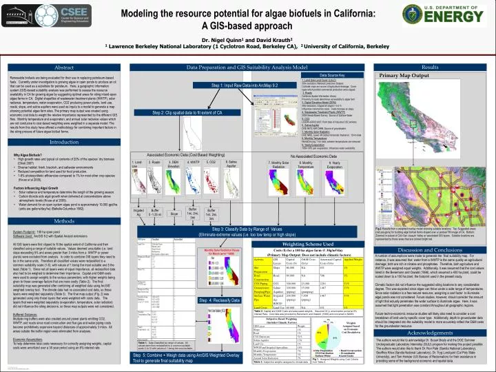
Modeling the resource potential for algae biofuels in California: A GIS-based approach Dr. Nigel Quinn1 and David Krauth2 1 Lawrence Berkeley National Laboratory (1 Cyclotron Road, Berkeley CA), 2 University of California, Berkeley Results Data Preparation and GIS Suitability Analysis Model Abstract Primary Map Output Renewable biofuels are being evaluated for their use in replacing petroleum-based fuels. Currently under investigation is growing algae in open ponds to produce an oil that can be used as a substitute for petroleum. Here, a geographic information system (GIS)-based suitability analysis was performed to assess the resource availability in CA for growing algae by suggesting optimal areas for siting inland-open algae farms in CA. Digital shapefiles of wastewater treatment plants (WWTP), solar radiance, temperature, water evaporation, CO2 producing power plants, land use, roads, slope, and saline aquifers were used as inputs to a model to generate a map showing potential algae farm sites. The primary map output was created using economic cost data to weight the relative importance represented by the different GIS files. Monthly temperature and evaporation, and annual solar radiance values which are not conducive to cost-based weighting were weighted in a separate model. The results from this study have offered a methodology for combining important factors in the siting process of future algae biofuel farms. Data Source Key 1. Land Use-Land Cover (LULC) 30m resolution; National Landcover Dataset Cultivate crops are source of agricultural drainage. Cover types which prohibit commercial production were clipped. 2. Roads California Spatial Information Library Proximity to roads determines accessibility to algae farm 3. Digital Elevation Model (DEM) 30m resolution, Clipped all slopes > 5.0 % Influences construction costs. Costs increase w/ slope. 4. Wastewater Treatment Plants (WWTP) 2004 Needs-Based Survey. Source of Surface-Water 5. CO2 USEPA eGRID 2007; Point data of industrial CO2 emitters 6. Saline Aquifer DOE NETL NATCARB; Source of groundwater. 7. Monthly Solar Radiation DOE NREL Lower 48 Global Horizontal Irradiance; 10 km data 8. Monthly Temperature WorldClim.org; 1 km data; extreme temperatures are removed 9. Yearly Evaporation 1956-1970 pan evaporation; influences water availability Step 1: Input Raw Data into ArcMap 9.2 Step 2: Clip spatial data to fit extent of CA Introduction Associated Economic Data (Cost Based Weighting) • Why Algae Biofuels? • High growth rates and typical oil contents of 20% of the species’ dry biomass • (Chisti 2007) • Diverse habitat: fresh, brackish, and saltwater environments • Reduced competition for land used for food production. • 1-8% photosynthetic efficiencies compared to 1% for most other crop species • (Kruse et al 2005). • Factors Influencing Algal Growth • Solar radiance and temperature determine the length of the growing season. • Carbon dioxide aids algal growth when delivered at concentrations above • atmospheric levels (Kruse et al 2005). • Water demand for an open system algae pond is approximately 10,000 gpd/ha (units are gallons/day/ha) (Battelle-Columbus 1982). No Associated Economic Data 6. SalineAquifer 5. CO2 1. Land- Use \ 3. DEM Elevation 4. WWTP 2. Roads 7. Monthly Solar Radiation 8. Monthly Temperature 9. Yearly Evaporation Buffer 1mi, 2mi, 3mi Irrigated Ag Buffer 0 -1.25 mi Buffer 1mi, 2mi, 3mi Slope Methods System Footprint : 100 ha open pond Software Used: ArcGIS 9.2 with Spatial Analyst extensions All GIS layers were first clipped to fit the spatial extent of California and then classified using a range of suitable values. Values deemed unsuitable (i.e. land slope exceeding 5% and areas greater than 3 miles from a WWTP or power plants) were excluded from analysis. In order to combine GIS layers they need to be in the same units. Therefore all classified values were reclassified to a common suitability scale (1-5), with values of 1 being the most suitable and 5 the least (Table 1). Since not all layers were of equal importance, all reclassified data also had to be weighed to determine their importance. Capital and O&M costs were used to assign weights to the various parameters, with higher weights being given to those coverage factors that are more costly (Table 2). The final suitability map was generated after combining all weighted data using ArcGIS’ weighted overlay tool. The climate data had no associated cost data, so those layers were weighted separately (Table 3). The final map output (Fig. 2) was generated using only those layers that were weighted with costs data. The layers that were weighted separately (evaporation, temperature, solar radiation) did not influence the siting decisions, so those map outputs were not considered. Buffered Distances Multiple ring buffers were also created around power plants emitting CO2, WWTP, and roads since road construction and flue gas and water piping costs become prohibitively expensive beyond distances of approximately 3 miles. All areas outside the buffer region were eliminated from analyses. Economic Assumptions To help determine total costs necessary for correctly assigning weights, capital costs were amortized over a 30 year period using an 8% interest rate. Step 3: Classify Data by Range of Values (Eliminate extreme values (i.e. too low temp or high slope) Fig 2. Results from a weighted overlay model showing suitable locations. Top: Suggested areas (red polygons) for building algal biofuel farms draped over a Landsat TM image of CA. Bottom: Zoomed in subset of CA’s San Joaquin Valley w/ associated GIS layers. Suitable locations are represented by those areas that are colored bright red. Weighting Scheme Used Discussion and Conclusions Monthly Solar Radiation Values for March (w/m2 *1000) A number of assumptions were made to generate the final suitability map. For instance, it was assumed that water from a WWTP is the same quality as agricultural drainage; both are rich in nitrates and phosphates. Therefore, both agriculture and WWTP were assigned equal weights. Additionally, it was assumed that the cost values listed in the Benemann and Oswald (1996), which assumed a 400 ha plant, could be scaled down to a 100 ha plant, the footprint used in the present study. Climatic factors did not influence the suggested siting locations to any considerable degree. This was expected since algae can thrive under a wide range of temperatures. Since solar radiation is a free natural resource, assigning a cost factor to illuminate algal ponds was not considered. Future studies, however, should consider the amount of light that actually penetrates the water surface to illuminate algae. Here, it was assumed that light penetration was constant throughout all geographic regions. Future techno-economic resource studies will likely also need to consider a cost breakdown of land use by specific cover type. Additionally, depth to groundwater data should be integrated into the suitability model to more accurately reflect the O&M costs for the groundwater resource. Step 4: Reclassify Data Acknowledgements The authors would like to acknowledge Dr. Susan Brady and the DOE Summer Undergraduate Laboratory Internship (SULI) program for making this project possible. The authors would also like to thank Dr. Ron Pate (Sandia National Laboratory), Geoffrey Klise (Sandia National Laboratory), Dr. Tryg Lundquist (Cal Poly State University), and Tom Heinzer (US Bureau of Reclamation) for their assistance in providing some of the background economic and spatial data. Step 5: Combine + Weigh data using ArcGIS Weighted Overlay Tool to generate final suitability map