Download

1 / 40
410 likes | 706 Views
Continuous Probability Distributions. Chapter 8. Introduction. A continuous random variable has an uncountable infinite number of values in the interval (a,b). The probability that a continuous variable X will assume any particular value is zero . . Area = 1.

E N D
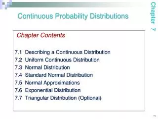
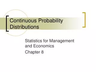
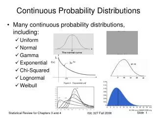
Continuous Probability Distributions Chapter 8
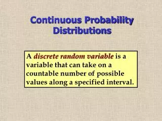
Introduction • A continuous random variable has an uncountable infinite number of values in the interval (a,b). • The probability that a continuous variable X will assume any particular value is zero.
Area = 1 8.1 Probability Density Function • To calculate probabilities of continuous random variables we define a probability density function f(x). • The density function satisfies the following conditions • f(x) is non-negative, • The total area under the curve representing f(x) is equal to 1.
a b Probability Density Function • The probability that x falls between ‘a’ and ‘b’ is found by calculating the area under the graph of f(x) between ‘a’ and ‘b’. P(a£x£b)
Uniform Distribution • A random variable X is said to be uniformly distributed if its density function is • The expected value and the variance are
Uniform Distribution The name is derived from the graph that describes this distribution f(X) X a b
Uniform Distribution • Example 8.1 • The daily sale of gasoline is uniformly distributed between 2,000 and 5,000 gallons. Find the probability that sales are: Between 2,500 and 3,500 gallon f(x) = 1/(5000-2000) = 1/3000 for x: [2000, 5000] P(2500£X£3000) = (3000-2500)(1/3000) = .1667 1/3000 x 2000 2500 3000 5000
Uniform Distribution • Example 8.1 • The daily sale of gasoline is uniformly distributed between 2,000 and 5,000 gallons. Find the probability that sales are: f(x) = 1/(5000-2000) = 1/3000 for x: [2000, 5000] More than 4,000 gallons P(X³4000) = (5000-4000)(1/3000) = .1333 1/3000 x 2000 4000 5000
Uniform Distribution • Example 8.1 • The daily sale of gasoline is uniformly distributed between 2,000 and 5,000 gallons. Find the probability that sales are: f(x) = 1/(5000-2000) = 1/3000 for x: [100,180] Exactly 2,500 gallons P(X=2500) = (2500-2500)(1/3000) = 0 1/3000 x 2000 2500 5000
8.2 Normal Distribution • A random variable X with mean m and variance s2is normally distributed if its probability density function is given by
The Shape of the Normal Distribution m The normal distribution is bell shaped, and symmetrical around m.
The effects of m and s The effects of m and s How does the standard deviation affect the shape of f(x)? s= 2 s =3 s =4 How does the expected value affect the location of f(x)? m = 10 m = 11 m = 12
m = 0 s = 1 Calculating Normal Probabilities • Two facts help calculate normal probabilities: • The normal distribution is symmetrical. • Any normal variable with some m and s can be transformed into a specific normal variable with m = 0 and s = 1, called…“STANDARD NORMAL DISTRIBUTION”
Calculating Normal Probabilities • Example 1 • The amount of time it takes to assemble a computer is normally distributed, with a mean of 50 minutes and a standard deviation of 10 minutes. • What is the probability that a computer is assembled in between 45 and 60 minutes?
Calculating Normal Probabilities • Solution • X denotes the assembly time of a computer. • Express P(45<X<60) in terms of Z. • We seek the probability P(45<X<60).
- m 45 - 50 X 60 - 50 s 10 10 (45-50)/10 = -.5 (60 – 50)/10 = 1 Calculating Normal Probabilities • Example 1 - continued P(45<X<60) = P( < < ) = P(-0.5<Z<1) To complete the calculation we need to compute the probability under the standard normal distribution
- m 45 - 50 X 60 - 50 P(45<X<60) = P( < < ) s 10 10 z0= -.5 z0 = 1 Calculating Normal Probabilities • Example 1 - continued = P(-.5<Z<1) We need to find the shaded area
Calculating Normal Probabilities • Example 1 - continued The probability provided by the Z-Table covers the area between ‘-infinity’ and some ‘z0’. z 0
Calculating Normal Probabilities Since we need to find the area between -0.5 and 1 (that is P(-.5<Z<1)) we’ll calculate the difference between P(-infinity<Z<1) <click> and P(-infinity<Z<-.5) <click> P(Z < 1) P(Z < -.5) z = 1 z= -.5 P(Z < 1) – P(Z<-.5)
Usding the Normal Table • Example 1 - continued = P(-.5<Z<1) = P(Z<1 .3413 0
Calculating Normal Probabilities • Example 1 - continued - P(Z< - .5) = .8413 - .3085 = P(-.5<Z<1) = P(Z<1
0% 10% Money is lost if the return is negative 0 - 10 5 P(Z< ) = P(Z< - 2) = .0228 Calculating Normal Probabilities Example 2: The rate of return (X) on an investment is normally distributed with mean of 10% and standard deviation of 5%. What is the probability of losing money? Solution (i) X P(X< 0 ) =
0% 10% Calculating Normal Probabilities • Solution(ii) – Example 2 ( 8.2) The curve for s =5% The curve for s = 10% X 0 - 10 10 (ii) P(X< 0 ) = P(Z< ) = P(Z< - 1) = .1587 Z Comment: When the standard deviation is 10% rather than 5%, more values fall away from the mean, so the probability of finding values at the distribution tail increases from .0228 to .1587.
Using Excel to Find Normal Probabilities • For P(X<k) enter in any empty cell: =normdist(k,m,s,True). • Example: Let m = 50 and s = 10. • P(X < 30): =normdist(30,50,10,True) • P(X > 45): =1 - normdist(45,50,10,True) • P(30<X<60): =normdist(60,50,10,True) – normdist(30,50,10,True). • Using “normsdist” • If the “Z” value is known you can use:P(Z<1.2234): =normsdist(1.2234)
Finding Values of Z • Sometimes we need to find the value of Z for a given probability • We use the notation zA to express a Z value for which P(Z > zA) = A A zA
A = .10 z.10 z.30 A3 = .95 - .40 = .55 1 – A = .70 A = .30 A1 = .95 A2 = .40 Finding Values of Z • Example 3: • What percentage of the standard normal population is located to the right of z.10?Answer: 10% • What percentage of the standard normal population is located to the left of z.30?Answer: 70% • What percentage of the standard normal population is located between z.95 and z.40: 55% Comment: z.95 has a negative value z.95 z.40
Finding Values of Z • Example 4 • Determine z exceeded by 5% of the population • Solution • z.05is defined as the z value for which the upper tail of the distribution is .05. Thus the lower tail is .95! .05 .04 .9495 .9505 1.6 0.05 0.95 1.645 Z0.05 0
0.05 Finding Values of Z • Example 4 • Determine z not exceeded by 5% of the population • Solution • Note we look for the z exceeded by 95% of the population. Because of the symmetry of the normal distribution it is the negative value of z.05! 0.95 1.645 -1.645 Z0.05 -Z0.05 0
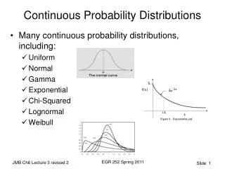
8.5 Other Continuous Distribution • Three new continuous distributions: • Student t-distribution • Chi-squared distribution • F distribution
The Student t - Distribution • The Student t density function n is the parameter of the student t – distribution E(t) = 0 V(t) = n/(n – 2) (for n > 2)
The Student t - Distribution n = 3 n = 10
Determining Student t Values • The student t distribution is used extensively in statistical inference. • Thus, it is important to determine the probability for any given value of the variable ‘t’ associated with a given number of degrees of freedom. • We can do this using • t tables • Excel
A A = .05 = .05 -tA Using the t - Table t t t t • The table provides the t values (tA) for which P(tn > tA) = A The t distribution is Symmetrical around 0 tA =-1.812 =1.812 t.100 t.05 t.025 t.01 t.005
The Chi – Squared Distribution • The Chi – Squared density function: • The parameter n is the number of degrees of freedom.
Determining Chi-Squared Values • Chi squared values can be found from the chi squared table or from Excel. • The c2-table entries are the c2 values of the right hand tail probability (A), for which P(c2n > c2A) = A. A c2A
A c2A Using the Chi-Squared Table To find c2 for which P(c2n<c2)=.01, lookup the column labeledc21-.01 or c2.99 =.05 A =.99 c2.05 c2.995 c2.990 c2.05 c2.010 c2.005
! ! ! The F Distribution • The density function of the F distribution:n1 and n2 are the numerator and denominator degrees of freedom.
The F Distribution • This density function generates a rich family of distributions, depending on the values of n1 and n2 n1 = 5, n2 = 10 n1 = 50, n2 = 10 n1 = 5, n2 = 10 n1 = 5, n2 = 1
Determining Values of F • The values of the F variable can be found in the F table or from Excel. • The entries in the table are the values of the F variable of the right hand tail probability (A), for which P(Fn1,n2>FA) = A.