Download
1 / 56
560 likes | 692 Views
Database Modelling. Lecture 5: Data Manipulation 2 Nick Rossiter. Learning Objectives. To consider the algebraic Cartesian Product operator; To consider the algebraic Generalised Join operator; To consider the algebraic Natural Join operator.

E N D
Database Modelling Lecture 5: Data Manipulation 2 Nick Rossiter
Learning Objectives • To consider the algebraic Cartesian Product operator; • To consider the algebraic Generalised Join operator; • To consider the algebraic Natural Join operator. • To consider the Natural & Generalised Joins using the SQL1 standard; • To consider the Natural & Generalised Joins using the SQL2 standard.
Requirement to Link Data together • Logically-related data • Held in different relations • Linked by Candidate Key/Foreign Key Relationships • Need to follow these relationships for retrieval • Need algebraic operator • To take a foreign key value and look it up as a candidate key in another table • This operator is called a join • There are many types of join but all typically involve candidate key and foreign key matches
Each arrow shows a Foreign Key/ Candidate Key link
Cartesian Product • is the simplest and crudest way to join 2 relations into one. • For 2 relations R and S, this can be expressed as : RCProdS • Cartesian Product creates a new relation • whose tuples are formed by merging • every tuple of the first operand with every tuple of the second operand, • that is all possible combinations of tuples.
Cartesian Product 2 • Is a primitive operator included for theoretical reasons. • The far more useful join operators that we will consider next are not primitive operators. • They are the equivalent of the (possible Projection of the) Restriction of a Cartesian Product, • all three of which are primitive operations, • i.e. cannot be implemented by an expression involving any more basic or more fundamental operator(s).
Size of Result of Cartesian Product Output is vast: product of size of the two operands
Examples of Result Sizes • While being rarely directly useful, Cartesian Product is always huge! • In particular its cardinality is the product of the operands’ cardinality. • For example operand cardinalities of: • 5 and 10 tuples yield a result cardinality of 50 tuples. • 25 and 50 yield a result cardinality of 1250 tuples. • 100 and 500 yield a result cardinality of 50,000 tuples. • 500 and 5,000 yield a result cardinality of 2,500,000. • The result size increases very rapidly.
Example of a Generalised Join (1) The Generalised Join operator still considers every tuple in one operand with every tuple in the other operand, just as Cartesian Product does. However, whereas Cartesian Product merges every combination, Generalised Join applies the condition provided as a parameter to each pair of tuples, and only if the condition is true does it copy the merged tuples into the result relation. Attribute B in relation R’s tuple is compared with attribute C in relation S’s tuple, and only if B in R is less than C in S are the 2 tuples merged and copied into the result.
Definition of Generalised Join • Creates a new relation which has all the attributes from both the operands; • the attributes retain their original names. • The result is created by : • looking at all possible combinations of tuples from the two operands. • using the comparison given as a parameter to compare each possible pair of tuples. • IF the comparison is trueTHEN the two tuples are merged into one tuple and copied into the resultELSE the two tuples are ignored
Definition of Generalised Join 2 • The new relation contains only the merged tuples. • The operator is also known as Theta Join. • The comparison provides a means of matching together tuples in the two different relations, • so that only matched tuples, i.e. related tuples, are copied into the result. • this is far more useful than Cartesian Product because it is normally related data that we want.
Definition of Generalised Join 3 A Generalised Join is equivalent to a Restriction of a Cartesian Product : R Gen[ condition ] S R CProd S Restrict[ condition ]
Join Conditions • The same attribute name cannot appear in both operands. • The two attributes compared in a condition must : • have the same data type • be in different relations • Condition can use any possible comparison that is permissible for values of that type. • Comparisons can be combined together with Boolean Operators (i.e. AND, OR, and NOT).
Theta Join • This alternative name for generalised join comes from mathematics. • The comparison provides a means of matching together tuples in the two different relations • far more useful than Cartesian Product because it is normally related data that we want. • all attributes from both tuples are used to form one new tuple. • the 2 original tuples cannot have any attribute names in common
Formal Definition A Generalised Join is equivalent to a Restriction of a Cartesian Product : R Gen[ condition ] S R CProd S Restrict[ condition ]
Join Conditions • The same attribute name cannot appear in both operands • The two attributes compared in a condition must : • have the same data type so that it is possible to compare them • be in different relations. • The condition can use any possible valid comparison for the types • Composite conditions can be formed using Boolean Operators.
Example of a Generalised Join (2) Every pair of tuples is matched by seeing whether attribute A in relation R is larger than attribute E in relation S AND whether attribute B in relation R is different to attribute D in relation S.
Size of Result of Generalised Join The result of a Generalised Join is as big as the result of a Cartesian Product in terms of the degree of the result. However in terms of cardinality, the result of a Generalised Join is usually much smaller than that of a Cartesian Product. But it depends on how many tuples match the join condition.
Example of an Equi Join (1) A single ‘=’ comparison is used, matching an employee with a car owner; i.e. we need the same employee number for both. The two attributes Owner and ENo are guaranteed to have duplicate data because an ‘=’ comparison was used to match the tuples.
Candidate Key/Foreign Key match • In a well-designed DB, it is frequently the case that the attributes to be compared in an Equi Join comprise a candidate key and its corresponding foreign key.
Example of Equi Join (2) SNo is a candidate key in SUPP and a foreign key in SHIP, whose only candidate key is (SNo, PNo). The result shows both problems, that of duplicate attribute names and that of duplicate data. The duplicate attribute names appear in the result because the attributes containing the same data in the two relations have the same name (not surprisingly).
The Two Equi Join Problems • Duplicate attribute names in the result • because attributes containing the same data in different relations usually have the same names. • Duplicate data in the result • due to the ‘=‘ comparison. • Yet the need for equals comparisons is very common.
Solution One • Rename the duplicate attribute(s) in one operand to something unique. • This solves the duplicate name problem. • Then do an equi join. • Use a Projection operation to remove the duplicate attribute data.
Solution TwoUse a Natural Join operator. • The Natural Join operator is effectively a non-primitive operator that carries out ‘Solution One’ • and so is effectively a short-hand for it. • Although Natural Join is a rather specialised operator compared to the Generalised Join, in fact it is used for at least 95% of joins • because of the common need for ‘=’ comparisons; • Generalised Join is used comparatively infrequently.
Definition of Natural Join • A special case of an Equi Join where: • all the attribute(s) to be compared must have the same name(s) and the same data type(s), • the duplicate attribute(s) are automatically removed from the result by the operator. • If there are duplicate attribute names in the operands, but they are not to be compared and used in the join, • a Natural Join operation will not do.
Example of Natural Join The Natural Join does what is most frequently required in a way that is simple and straightforward for the user, hence the name “natural”. Problem solved, with elegance!
So Two Basic Types of Join Operator Natural Join RJoin [ attribute name(s) ] S Generalised Join RGen [ condition ] S Equi join is readily expressed by a Generalised Join
Joins in SQL • Expressing joins in SQL has been particularly affected by two SQL standards: • SQL1 Standard SQL, introduced in 1989 - this has no explicit support for joins • No join operation • Achieve effect of join with WHERE clause • SQL2 Standard SQL, introduced in 1992 - this has explicit support for joins • Join operation
SQL1 : Generalised Join Syntax The Generalised Join of relations R and S has the syntax: Principles : Put Select * to get all the attributes in the result. Put both relation names in the From phrase. Put the theta join condition in the Where phrase.
SQL result • The result has all the columns from both tables. • SQL is forgiving in that if the two tables have duplicate column names • both appear in the result and • can be distinguished from each other • because the column names are prefixed with their table names. • In a single database, this is always unique: • table_name.attribute_name
SQL1 as Natural Join • SQL1 fulfills all the requirements of the Natural Join operation. • The user has to manually enter all the result columns from both tables into the Select phrase, omitting duplicate columns. • Although the ‘=’ comparison means that it does not matter which duplicate column appears in the result • user must arbitrarily prefix the common column name with one table name
Example : SQL1 Generalised Joins SQL1 equivalents of previous examples As the operands have no column names in common, it is safe to use * in the Select phrase and omit table-name prefixes in the Where phrase.
Example : SQL1 Natural Join SQL1 equivalent of previous example
Combining Algebra Operators • Typically we want to join together 2 relations holding relevant data, • and then prune the result down with • projection and • restriction • to yield just the required data:
General Format SQL Query In SQL, put the Projected attributes in the Select phrase, the Joined relations in the From phrase, and And the Join and Restrict conditions together in the Where phrase, as follows : Include the Distinct keyword to be on the safe side. Select Distinct AttNames From R, S Where ( R.Att = S.Att ) And (condition ) ; SQL’s built-in sequence of operations will execute a Cartesian Product of R and S, then a Restrict on the result using the entire Where condition, and finally a Project on that result using the Select attributes.
Examples of Combining Operators 1 Example 1: Get the supplier’s name who supplies parts in quantities of 10. SHIP Join[ SNo ] SUPP Restrict[ Qty = 10 ] Project[ SName ] Select Distinct Sname From SHIP, SUPP Where SHIP.SNo = SUPP.SNo And Qty = 10 ; Note that column names have only been prefixed with table names where this is a logical necessity, as in the Natural Join condition of the example above.
Examples of Combining Operators 2 Example 2: Get the names of employees who own a Corsa 1.3. CAR Gen[ Owner = ENo ] EMPLOYER Restrict[ Type = ‘Corsa 1.3’ ] Project[ EName ] Select Distinct EName From CAR, EMPLOYEE Where Owner = ENo And Type = ‘Corsa 1.3’ ;
Designing SQL Queries • Decide which DB relations contain data that will be required in the answer to the query • join all those relations together with the appropriate Natural/GeneralisedJoin operation. • Remove any unrequired tuples with Restrict operation(s) as a filter. • Remove any unrequired attributes with a Project operation.
SQL : Cartesian Product SQL1 executes a Cartesian Product operation given the following syntax Hence the absence of a join condition in the Where phrase causes SQL to execute a Cartesian Product : If a Join condition is accidentally omitted from the Where phrase by error, then the result will be unexpectedly (very) large due to a Cartesian Product operation !
SQL Join -- Algebra Style • SQL2 uses an algebra-like style to fulfill the Generalised Join requirements • Thus everything to do with a Join operation is written succinctly in one place • in the From phrase. • Simpler to use • Should be preferred way of writing Generalised Joins wherever SQL2 syntax is available.
Example : SQL2 Generalised Joins SQL2 equivalents of previous examples As the operands have no column names in common, it is safe to use * in the Select phrase and omit table name prefixes in the Where phrase.
SQL2 : Natural Join Syntax There are 2 ways of writing a Natural Join of operands R and S in SQL2 Principles : These are the same as for Generalised Join, except that a different required expression is put in the From phrase.
Examples : SQL2 Natural Joins SQL2 equivalents of a previous example
Pros and Cons of the Two Syntaxes 1 R Natural Join S • Advantage : less to write. • Disadvantage : easier to make a mistake if the required comparable columns don’t exist. • Use for interactive ad hoc queries where it is easy to recover from a mistake.