Download
1 / 40
470 likes | 573 Views
2 Eddy Current Theory. 2.1 Eddy Current Method 2.2 Impedance Measurements 2.3 Impedance Diagrams 2.4 Test Coil Impedance 2.5 Field Distributions. 2.1 Eddy Current Method. 1. 1. f = 0.05 MHz. f = 0.05 MHz. 0.8. 0.8. f = 0.2 MHz. f = 0.2 MHz. 0.6. 0.6. f = 1 MHz. f = 1 MHz.

E N D
2 Eddy Current Theory 2.1 Eddy Current Method 2.2 Impedance Measurements 2.3 Impedance Diagrams 2.4 Test Coil Impedance 2.5 Field Distributions
1 1 f = 0.05 MHz f = 0.05 MHz 0.8 0.8 f = 0.2 MHz f = 0.2 MHz 0.6 0.6 f = 1 MHz f = 1 MHz 0.4 0.4 0.2 0.2 0 0 | F | Re { F} -0.2 -0.2 0 0 1 1 2 2 3 3 Depth [mm] Depth [mm] Eddy Current Penetration Depth δ standard penetration depth aluminum (σ = 26.7 106 S/m or 46 %IACS)
primary magnetic flux primary (excitation) current secondary secondary (eddy) current magnetic flux Eddy Currents, Lenz’s Law
Ze Zp Vp Ve Impedance Measurements Current generator: Zp Vp Ie Voltage divider: Ie
R C L Vo Ve 1 Q = 2 0.8 Q = 5 Q = 10 0.6 Transfer Function, |K| 0.4 0.2 0 0 1 2 3 Normalized Frequency, w/W Resonance
Z1 Z4 + G Ve _ V2 Z2 Z3 Wheatstone Bridge probe coil reference coil R0 reference resistance Lc reference (dummy) coil inductance Rc reference coil resistance L* complex probe coil inductance
0.5 0.4 0.3 Transfer Function, | K0 | 0.2 Lc = 100 µH Lc = 20 µH 0.1 Lc = 10 µH 0 0 1 2 3 Frequency [MHz] Impedance Bandwidth R0 = 100 Ω, Rc = 10 Ω
Im(Z) Im(Z) Im(Z) Im(Z) Re(Z) Re(Z) Re(Z) Re(Z) Ω- 0 ∞ Ω+ Examples of Impedance Diagrams Ω- L L R R 0 ∞ C C Ω+ R2 R R1 0 0 Ω Ω L L R1 R ∞ ∞ R1+R2 C C
I I I I 2 2 1 1 V N N V 1 2 1 2 F F F F , 11 12 21 22 V V L , L , L 1 2 11 12 22 Magnetic Coupling
I I 2 1 V V L , L , L R 1 2 11 12 22 e Probe Coil Impedance
1 0.9 0.8 Re=30 W 0.7 0.6 0.5 Normalized Reactance 0.4 Re=10 W 0.3 0.2 κ = 0.6 Re=5 W κ = 0.8 0.1 κ = 0.9 0 0 0.1 0.2 0.3 0.4 0.5 Normalized Resistance Impedance Diagram lift-off trajectories are straight: conductivitytrajectories are semi-circles
0.42 0.42 0.40 0.40 0.38 0.38 “Vertical” Impedance Component 0.36 0.36 0.34 0.34 0.32 0.32 0.28 0.28 0.3 0.3 0.32 0.32 0.34 0.34 0.36 0.36 0.38 0.38 “Horizontal” Impedance Component Electric Noise versus Lift-off Variation “physical” coordinates rotated coordinates lift-off lift-off Normalized Reactance Normalized Resistance
0.14 0.42 0.12 0.40 0.10 lift-off 0.38 0.08 Gauge Factor, F 0.06 0.36 Normalized Reactance 0.04 absolute 0.34 0.02 normal 0 0.32 0.28 0.3 0.32 0.34 0.36 0.38 0 0.2 0.4 0.6 0.8 1 Frequency [MHz] Normalized Resistance Conductivity Sensitivity, Gauge Factor
1 1 0.9 0.9 0.8 0.8 0.7 0.7 0.6 0.6 lift-off 0.5 0.5 κ 0.4 0.4 κ lift-off Normalized Reactance Normalized Reactance 0.3 0.3 0.2 0.2 0.1 0.1 conductivity conductivity 0 0 0 0 0.1 0.1 0.2 0.2 0.3 0.3 0.4 0.4 0.5 0.5 Normalized Resistance Normalized Resistance Conductivity and Lift-off Trajectories finite probe size conductivity trajectories are not semi-circles lift-off trajectories are not straight
a coil radius L coil length Air-core Probe Coils single turn L = a L = 3 a
z + Js _Js for inside loops (r1,2 < a) inside loop encircling outside loop L for outside loops (r1,2 > a) 2a for encircling loops (r1 < a < r2) Infinitely Long Solenoid Coil
+ Js _Js z 2 b 2 a Magnetic Field of an Infinite Solenoid with Conducting Core in the air gap (b < r < a) Hz = Js in the core (0 < r < b) Hz = H1J0(kr) Jnnth-order Bessel function of the first kind
z 2 b 2 a Magnetic Flux of an Infinite Solenoid with Conducting Core + Js _Js
Impedance of an Infinite Solenoid with Conducting Core For an empty solenoid (b = 0): Normalized impedance:
1.2 real part 1.0 imaginary part 0.8 0.6 g-function 0.4 0.2 0.0 -0.2 -0.4 0.01 0.1 1 10 100 1000 Normalized Radius, b/δ Resistance and Reactance of an Infinite Solenoid with Conducting Core
1 b/δ = 1 0.8 2 0.7 0.6 lift-off 0.8 Normalized Reactance 3 a 0.4 0.9 w κ = 1 5 0.2 10 20 0 0 0.1 0.2 0.3 0.4 0.5 Normalized Resistance Effect of Changing Coil Radius lift-off a (changes) b (constant)
1 0.8 lift-off a (constant) 0.6 0.4 b (changing) 0.2 0 0 0.1 0.2 0.3 0.4 0.5 Effect of Changing Core Radius wn = 4 0.7 lift-off 0.8 Normalized Reactance 9 b 0.9 w κ = 1 25 100 400 Normalized Resistance
4 µr = 4 ωn = 0.6 3 1 ω µ 3 1.5 Normalized Reactance 2 2 1 1 0 0 0.2 0.4 0.6 0.8 1 1.2 Normalized Resistance Permeability
a c b a b Solid Rod versus Tube solid rod BC1: continuity of Hz at r = b tube BC1: continuity of Hz at r = b BC2: continuity of Hz at r = c BC3: continuity of Eφ at r = c
1 a thick tube 0.8 σ1 c b 0.6 Normalized Reactance solid rod σ2 σ1 0.4 very thin tube σ2 0.2 0 Normalized Resistance 0 0.1 0.2 0.3 0.4 0.5 0.6 Solid Rod versus Tube
1 0.8 b/ = 2 η = 0 solid rod 0.6 b/ = 3 a Normalized Reactance η = 0.2 η = 0.4 η = 0.6 0.4 c η = 0.8 b/ = 5 b 0.2 b/ = 10 b/ = 20 η 1 thin tube 0 0 0.1 0.2 0.3 0.4 0.5 0.6 Normalized Resistance Wall Thickness
thin tube κ = 0.95, η = 0.99 solid rod κ = 1, η = 0 1 solid rod κ = 0.95, η = 0 0.8 Normalized Reactance a 0.6 c b 0.4 thin tube κ = 1, η = 0.99 0.2 Normalized Resistance 0 0 0.1 0.2 0.3 0.4 0.5 0.6 Wall Thickness versus Fill Factor
1 0.8 0.6 0.4 0.2 0 0 0.1 0.2 0.3 0.4 0.5 0.6 Clad Rod master curve for solid rod lower fill factor solid brass rod Normalized Reactance a d brass cladding on copper core copper cladding on brass core solid copper rod d b c thin wall Normalized Resistance
2ao 2ai h ℓ t Dodd and Deeds. J. Appl. Phys. (1968) 2D Axisymmetric Models a pancake coil (2D) c b short solenoid (2D) ↓ long solenoid (1D) ↓ thin-wall long solenoid (≈0D) ↓ coupled coils (0D)
0.2 1 coil diameter 4 mm 0.8 0.15 2 mm 1 mm 0.6 lift-off 0.1 fM 0.1 mm Normalized Reactance (Normal) Gauge Factor 0.4 0.05 mm 0.05 0.2 frequency 0 mm 0 0 0.1 1 10 100 0 0.05 0.1 0.15 0.2 0.25 0.3 Normalized Resistance Frequency [MHz] a0 = 1 mm, ai = 0.5 mm, h = 0.05 mm, = 1.5 %IACS, = 0 Flat Pancake Coil (2D)
electric field Eθ magnetic field (eddy current density) 10 Hz 10 kHz 1 MHz 10 MHz 1 mm air-core pancake coil (ai = 0.5 mm, ao = 0.75 mm, h = 2 mm), in Ti-6Al-4V (σ = 1 %IACS) Field Distributions
101 standard actual 100 ai Axial Penetration Depth, δa [mm] 10-1 10-2 10-5 10-4 10-3 10-2 10-1 100 101 102 Frequency [MHz] air-core pancake coil (ai = 0.5 mm, ao = 0.75 mm, h = 2 mm) in Ti-6Al-4V Axial Penetration Depth
2.0 analytical finite element 1.8 1.6 1.4 1.2 1.0 0.8 10-5 10-4 10-3 10-2 10-1 100 101 102 Frequency [MHz] air-core pancake coil (ai = 0.5 mm, ao = 0.75 mm, h = 2 mm) in Ti-6Al-4V Radial Spread Radial Spread, as [mm]
101 standard actual 100 10-1 10-2 10-5 10-4 10-3 10-2 10-1 100 101 102 Frequency [MHz] air-core pancake coil (ai = 0.5 mm, ao = 0.75 mm, h = 2 mm) in Ti-6Al-4V Radial Penetration Depth Radial Penetration Depth, δr [mm]
1.8 FE prediction 1.6 experimental 1.4 1.2 1.0 Radial Spread, as [mm] 0.8 0.6 0.4 0.2 0 10-2 10-1 100 101 Frequency [MHz] ferrite-core pancake coil (ai = 0.625 mm, ao = 1.25 mm, h = 3 mm) in Ti-6Al-4V Lateral Resolution