Download

1 / 62
620 likes | 626 Views
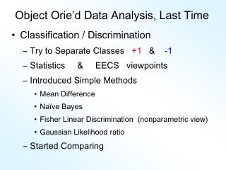
Object Orie’d Data Analysis, Last Time. Organizational Matters http://www.unc.edu/~marron/UNCstat322-2005/HomePage.html What is OODA? Visualization by Projection Object Space & Feature Space Curves as Data Data Representation Issues PCA visualization. Data Object Conceptualization.

E N D
Object Orie’d Data Analysis, Last Time • Organizational Matters http://www.unc.edu/~marron/UNCstat322-2005/HomePage.html • What is OODA? • Visualization by Projection • Object Space & Feature Space • Curves as Data • Data Representation Issues • PCA visualization
Data Object Conceptualization Object Space Feature Space Curves Images Manifolds Shapes Tree Space Trees
Easy way to do these analyses • Matlab software (user friendly?) available: • http://www.stat.unc.edu/postscript/papers/marron/Matlab7Software/ • Download & put in Matlab Path: • General • Smoothing • Look first at: • curvdatSM.m • scatplotSM.m
Time Series of Curves • Again a “Set of Curves” • But now Time Order is Important! • An approach: Use color to code for time Start End
Time Series Toy E.g. Explore Question of Eli Broadhurst: “Is Horizontal Motion Linear Variation?” Example: Set of time shifted Gaussian densities View: Code time with colors as above
T. S. Toy E.g., PCA View PCA gives “Modes of Variation” But there are Many… Intuitively Useful??? Like “harmonics”? Isn’t there only 1 mode of variation? Answer comes in 2-d scatterplots
T. S. Toy E.g., PCA Scatterplot • Where is the Point Cloud? • Lies along a 1-d curve in • So actually have 1-d mode of variation • But a non-linear mode of variation • Poorly captured by PCA (linear method) • Will study more later
Chemo-metric Time Series • Mass Spectrometry Measurements • On an Aging Substance, called “Estane” • Made over Logarithmic Time Grid, n = 60 • Each is a Spectrum • What about Time Evolution? • Approach: PCA & Time Coloring
Chemo-metric Time Series • Joint Work w/ E. Kober & J. Wendelberger • Los Alamos National Lab • Four Experimental Conditions: • Control • Aged 59 days in Dry Air • Aged 27 days in Humid Air • Aged 59 days in Humid Air
Chemo-metric Time Series, HA 27 • Raw Data: • All 60 spectra essentially the same • “Scale” of mean is much bigger than variation about mean • Hard to see structure of all 1600 freq’s • Centered Data: • Now can see different spectra • Since mean subtracted off • Note much smaller vertical axis
Chemo-metric Time Series, HA 27 • Data zoomed to “important” freq’s: • Raw Data: • Now see slight differences • Smoother “natural looking” spectra • Centered Data: • Differences in spectra more clear • Maybe now have “real structure” • Scale is important
Chemo-metric Time Series, HA 27 • Use of Time Order Coloring: • Raw Data: • Can see a little ordering, not much • Centered Data: • Clear time ordering • Shifting peaks? (compare to Raw) • PC1: • Almost everything? • PC1 Residuals: • Data nearly linear (same scale import’nt)
Chemo-metric Time Series, Control • PCA View • Clear systematic structure • Time ordering very important • Reminiscent of Toy Example • A clear 1-d curve in Feature Space • Physical Explanation?
Toy Data Explanations • Simple Chemical Reaction Model: • Subst. 1 transforms into Subst. 2 • Note: linear path in Feature Space
Toy Data Explanations • Richer Chemical Reaction Model: • Subst. 1 Subst. 2 Subst. 3 • Curved path in Feat. Sp. • 2 Reactions Curve lies in 2-dim’al subsp.
Toy Data Explanations • Another Chemical Reaction Model: • Subst. 1 Subst. 2 & Subst. 5 Subst. 6 • Curved path in Feat. Sp. • 2 Reactions Curve lies in 2-dim’al subsp.
Toy Data Explanations • More Complex Chemical Reaction Model: • 1 2 3 4 • Curved path in Feat. Sp. (lives in 3-d) • 3 Reactions Curve lies in 3-dim’al subsp.
Toy Data Explanations • Even More Complex Chemical Reaction Model: • 1 2 3 4 5 • Curved path in Feat. Sp. (lives in 4-d) • 4 Reactions Curve lies in 4-dim’al subsp.
Chemo-metric Time Series, Control • Suggestions from Toy Examples: • Clearly 3 reactions under way • Maybe a 4th??? • Hard to distinguish from noise? • Interesting statistical open problem!
Chemo-metric Time Series • What about the other experiments? Recall: • Control • Aged 59 days in Dry Air • Aged 27 days in Humid Air • Aged 59 days in Humid Air • Above results were “cherry picked”, • to best makes points • What about cases???
Scatterplot Matrix, Control Above E.g., maybe ~4d curve ~4 reactions
Scatterplot Matrix, Da59 PC2 is “bleeding of CO2”, discussed below
Scatterplot Matrix, Ha27 Only “3-d + noise”? Only 3 reactions
Scatterplot Matrix, Ha59 Harder to judge???
Object Space View, Control Terrible discretization effect, despite ~4d …
Object Space View, Da59 OK, except strange at beginning (CO2 …)
Object Space View, Ha27 Strong structure in PC1 Resid (d < 2)
Object Space View, Ha59 Lots at beginning, OK since “oldest”
Problem with Da59 What about strange behavior for DA59? Recall: PC2 showed “really different behavior at start” Chemists comments: Ignore this, should have started measuring later…
Problem with Da59 But still fun to look at broader spectra
Chemo-metric T. S. Joint View • Throw them all together as big population • Take Point Cloud View
Chemo-metric T. S. Joint View • Throw them all together as big population • Take Point Cloud View • Note 4d space of interest, driven by: • 4 clusters (3d) • PC1 of chemical reaction (1-d) • But these don’t appear as the 4 PCs • Chem. PC1 “spread over PC2,3,4” • Essentially a “rotation of interesting dir’ns” • How to “unrotate”???
Chemo-metric T. S. Joint View Interesting Variation: Remove cluster means Allows clear comparison of within curve variation
Chemo-metric T. S. Joint View • Interesting Variation: • Remove cluster means • Allows clear comparison of within curve variation: • PC1 versus others are quite revealing • (note different “rotations”) • Others don’t show so much
Demography Data Joint Work with: Andres Alonso Univ. Carlos III, Madrid • Mortality, as a function of age • “Chance of dying”, for Males, in Spain • of each 1-year age group • Curves are years • 1908 - 2002 • PCA of the family of curves
Demography Data • PCA of the family of curves for Males • Babies & elderly “most mortal” (Raw) • All getting better over time (Raw & PC1) • Except 1918 - Influenza Pandemic • (seeColor Scale) • Middle age most mortal (PC2): • 1918 • Early 1930s - Spanish Civil War • 1980 – 1994 (then better) auto wrecks • Decade Rounding (several places)
Demography Data • PCA for Females in Spain • Most aspects similar • (seeColor Scale) • No War Changes • Steady improvement until 70s (PC2) • When auto accidents kicked in
Demography Data • PCA for Males in Switzerland • Most aspects similar • No decade rounding (better records) • 1918 Flu – Different Color (PC2) • (seeColor Scale) • No War Changes • Steady improvement until 70s (PC2) • When auto accidents kicked in
Demography Data • Dual PCA • Idea: Rows and Columns trade places • Demographic Primal View: • Curves are Years, Coord’s are Ages • Demographic Dual View: • Curves are Ages, Coord’s are Years Dual PCA View, Spanish Males
Demography Data Dual PCA View, Spanish Males • Old people have const. mortality (raw) • But improvement for rest (raw) • Bad for 1918 (flu) & Spanish Civil War, but generally improving (mean) • Improves for ages 1-6, then worse (PC1) • Big Improvement for young (PC2) • (Age Color Key)