Download
1 / 22
300 likes | 859 Views
High Throughput Sequencing. Xiaole Shirley Liu STAT115, STAT215, BIO298, BIST520. First Generation. Sanger Sequencing: sequencing and detection 2 different steps: 384 * 1kb / 3 hours. Second Generation. Massively parallel sequencing by synthesis

E N D
High Throughput Sequencing Xiaole Shirley Liu STAT115, STAT215, BIO298, BIST520
First Generation • Sanger Sequencing: sequencing and detection 2 different steps: 384 * 1kb / 3 hours
Second Generation • Massively parallel sequencing by synthesis • Many different technologies: Illumina, 454, SOLiD, Helicos, etc • Illumina: HiSeq, MiSeq, NextSeq • 1-16 samples • 25M-4B reads • 30-300bp • 1-8 days • 15GB-1TB output • Moving targets
Illumina Cluster Generation • Amplify sequenced fragments in place on the flow cell • Can sequence from both the pink and purple adapters (Paired-end seq) • Can multiplex many samples / lane
Third Generation • Single molecule sequencing: no amp • Fewer but much longer reads • Good for genome sequencing, but not for read count applications http://www.youtube.com/watch?v=v8p4ph2MAvI
High Throughput Sequencing • Big (data), fast (speed), cheap (cost), flexible (applications) • Bioinformatic analyses become bottleneck
FASTQ File • Format • Sequence ID, sequence • Quality ID, quality score • Quality score using ASCII (higher -> better) @HWI-EAS305:1:1:1:991#0/1 GCTGGAGGTTCAGGCTGGCCGGATTTAAACGTAT +HWI-EAS305:1:1:1:991#0/1 MVXUWVRKTWWULRQQMMWWBBBBBBBBBBBBBB @HWI-EAS305:1:1:1:201#0/1 AAGACAAAGATGTGCTTTCTAAATCTGCACTAAT +HWI-EAS305:1:1:1:201#0/1 PXX[[[[XTXYXTTWYYY[XXWWW[TMTVXWBBB
Read Mapping • Mapping hundreds of millions of reads back to the reference genome is CPU and RAM intensive and slow • Read quality decreases with length (small single nucleotide mismatches or indels) • Most mappers allow ~2 mismatches within first 30bp (4 ^ 28 could still uniquely identify most 30bp sequences in a 3GB genome), slower when allowing indels • Mapping output: SAM (BAM) or BED
Spaced seed alignment • Tags and tag-sized pieces of reference are cut into small “seeds.” • Pairs of spaced seeds are stored in an index. • Look up spaced seeds for each tag. • For each “hit,” confirm the remaining positions. • Report results to the user.
Burrows-Wheeler • Store entire reference genome. • Align tag base by base from the end. • When tag is traversed, all active locations are reported. • If no match is found, then back up and try a substitution. Trapnell & Salzberg, Nat Biotech 2009
Burrows-Wheeler Transform • Reversible permutation used originally in compression • Once BWT(T) is built, all else shown here is discarded • Matrix will be shown for illustration only T BWT(T) Encoding for compression gc$ac 1111001 Burrows Wheeler Matrix Last column Burrows M, Wheeler DJ: A block sorting lossless data compression algorithm. Digital Equipment Corporation, Palo Alto, CA 1994, Technical Report 124; 1994 Slides from Ben Langmead
Burrows-Wheeler Transform • Property that makes BWT(T) reversible is “LF Mapping” • ith occurrence of a character in Last column is same text occurrence as the ith occurrence in Firstcolumn Rank: 2 BWT(T) T Rank: 2 Burrows Wheeler Matrix Slides from Ben Langmead
Burrows-Wheeler Transform • To recreate T from BWT(T), repeatedly apply rule: T = BWT[ LF(i) ] + T; i = LF(i) • Where LF(i) maps row i to row whose first character corresponds to i’s last per LF Mapping FinalT Slides from Ben Langmead
Exact Matching with FM Index • To match Q in T using BWT(T), repeatedly apply rule: top =LF(top, qc); bot = LF(bot, qc) • Whereqc is the next character in Q (right-to-left) and LF(i, qc) maps row i to the row whose first character corresponds to i’s last character as if it were qc Slides from Ben Langmead
Exact Matching with FM Index • In progressive rounds, top & bot delimit the range of rows beginning with progressively longer suffixes of Q (from right to left) • If range becomes empty the query suffix (and therefore the query) does not occur in the text • If no match, instead of giving up, try to “backtrack” to a previous position and try a different base (mismatch, much slower) Slides from Ben Langmead
Seq Files @HWI-EAS305:1:1:1:991#0/1 GCTGGAGGTTCAGGCTGGCCGGATTTAAACGTAT +HWI-EAS305:1:1:1:991#0/1 MVXUWVRKTWWULRQQMMWWBBBBBBBBBBBBBB @HWI-EAS305:1:1:1:201#0/1 AAGACAAAGATGTGCTTTCTAAATCTGCACTAAT +HWI-EAS305:1:1:1:201#0/1 PXX[[[[XTXYXTTWYYY[XXWWW[TMTVXWBBB HWUSI-EAS366_0112:6:1:1298:18828#0/1 16 chr9 98116600 255 38M * 0 0 TACAATATGTCTTTATTTGAGATATGGATTTTAGGCCG Y\]bc^dab\[_UU`^`LbTUT\ccLbbYaY`cWLYW^ XA:i:1 MD:Z:3C30T3 NM:i:2 HWUSI-EAS366_0112:6:1:1257:18819#0/1 4 * 0 0 * * 0 0 AGACCACATGAAGCTCAAGAAGAAGGAAGACAAAAGTG ece^dddT\cT^c`a`ccdK\c^^__]Yb\_cKS^_W\ XM:i:1 HWUSI-EAS366_0112:6:1:1315:19529#0/1 16 chr9 102610263 255 38M * 0 0 GCACTCAAGGGTACAGGAAAAGGGTCAGAAGTGTGGCC ^c_Yc\Lcb`bbYdTa\dd\`dda`cdd\Y\ddd^cT` XA:i:0 MD:Z:38 NM:i:0 chr1 123450 123500 + chr5 28374615 28374615 - • Raw FASTQ • Sequence ID, sequence • Quality ID, quality score • Mapped SAM • Map: 0 OK, 4 unmapped, 16 mapped reverse strand • XA (mapper-specific) • MD: mismatch info • NM: number of mismatch • Mapped BED • Chr, start, end, strand http://samtools.sourceforge.net/SAM1.pdf
Mapping Statistics Terms • Mappable locations: reads that can find match to A location in the genome • Uniquely mapped reads: reads that can find match to A SINGLE location in the genome • Repeat sequences in the genome, length-dependent • Uniquely mapped locations: number of unique locations hit by uniquely mapped reads • Redundancy: potential PCR amplification bias
Summary • Sequencing technologies • 1st, 2nd, 3rd generation • Sequence quality assessment • FASTQC • Read mapping • Spaced seed • BWA: Borrows Wheeler transformation, LF mapping