Download
1 / 48
510 likes | 561 Views
Plant Breeding Lecture 3. Objectives. Know essential terminology Know some examples of traits targeted by breeding for genetic improvement of crops Understand the foundations of plant breeding Know breeding techniques. Gamete.

E N D
Objectives Know essential terminology Know some examples of traits targeted by breeding for genetic improvement of crops Understand the foundations of plant breeding Know breeding techniques
Gamete A mature reproductive cell that is specialized for sexual fusion Haploid (n) Cells that have only one set of chromosomes (n). Each gamete is haploid Cross A mating between two individuals, leading to the fusion of gametes and progeny Diploid (2n) Cells with two copies of each chromosome. The diploid state is attained by the fusion of two gametes Zygote The cell produced by the fusion of the male and female gametes
Gene The inherited segment of DNA that determines a specific characteristic in an organism Locus The specific place on the chromosome where a gene is located Alleles Alternative forms of a gene
Genotype The genetic constitution of an organism Homozygous An individual whose genetic constitution has both alleles the same for a given gene locus (i.e., AA or aa) Heterozygous An individual whose genetic constitution has different alleles for a given gene locus (i.e., Aa)
Homogeneous A population of individuals having the same genetic constitution (e.g., a field of pure-line soybean or a field of hybrid corn) Heterogeneous A population of individuals having different genetic constitutions Phenotype The physical manifestation of a genetic trait that results from a specific genotype and its interaction with the environment
Trait goals Yield = seeds, biomass, or fruit size/number Quality traits, such as oil, flavor, color Stress tolerance, e.g., drought Insect and disease resistance Introgressing transgenes into plant varieties
Yield Figure 3.5 Yield of hybrid corn varieties versus year of release. Data were obtained from Duvick and Cassman (1999), based on field experiments conducted at a plant density of 79,000 plants per hectare at three locations in central Iowa in 1994.
H H C C H H H C C H H H CC • Hydrogenation: flavor and oxidative stability • Trans fats: health issues • FDA label mandate Quality trait: oil quality cis form saturated trans form Hydrogenation ; (Source: Wilson, 2004)
Insect and disease resistance Soybean sudden death syndrome
Deployment of transgenic traits (e.g., transfer of herbicide resistant genes in commercial varieties)
Foundations of plant breeding Importance of genetic variation and selection
What are the causes of biological variation observed in plants? 1. Genetic causes (mode of inheritance) • single genes • multiple genes 2. Environmental 3. GxE: the interaction between the genotype of the plant and the environment in which it grows
Phenotype vs. Genotype P = G + E + (GxE) P is called the phenotypic value, i.e., the measurement associated with a particular individual G is genotypic value, the effect of the genotype (averaged across all environments) E is the effect of the environment (averaged across all genotypes)
The genotype responds more strongly in some environments. • Sets of environments tend to shift the trait value in one direction, other environments in a different direction. • If we could measure P in all possible environments and regard E as a deviation, then the mean of E would be zero and P = G.
Figure 3.8 Figure 3.8 In Sewall Wright’s shifting balance theory, a genotype or population is defined by coordinates in N-dimensional space, and a fitness value forms a surface in the (N + 1)th-dimension. Here, genotype coordinates are defined in two dimensions on the ground beneath a mountainous fitness surface (the third dimension). The coordinates of a given population can be changed by selection, but only in small increments. Direct selection tends to move a population toward coordinates where fitness is highest, but that may be only a local peak. Applying this concept to plant breeding, we see that to find genotypes beneath a global peak, we need to create and explore a large genotype space (i.e., genetic diversity) or to know exactly where we are going (an ideotype).
Methods and strategies: when and why each is useful Typically the goal is cultivar production
Qualitative traits, simple inheritance, controlled by major genes • Quantitative traits, complex inheritance controlled be several gene loci How complex is selection?
Qualitative traits • Classified into discrete classes • Individuals in each class counted • Someenvironmental influence on phenotype • Controlled by a few (<3) major genes
Mendel’s seven traits showing simple inheritance Figure 2.3 Often single gene traits are easy to see or measure, since environment typically has limited control over their expression Tawny (TT or Tt) versus gray (tt) single gene locus on soybean chromosome 6
Parent 1 Parent 1 Y y Y Y YY Yy Yy Yy Y y Parent 2 Parent 2 Yy yy y Yy Yy y Figure 2.4. A. Monohybrid Cross B. F1 Self Fertilization = Parent 1 Parent 2 Parent 2 Parent 1 X X Yy YY yy Yy Gametes: Y Y y y Gametes: Y y Y y F1 Fertilization: F2 Fertilization: YY & Yy Yy F2 Plants: 75% yellow 25% green F1 Hybrid Plants: 100% yellow yy
Gene and Genotype FrequenciesExample: Self pollinated diploid species Upon selfing F2 population; 25% homozygous ‘YY’ will produce only ‘YY’ genotypes, and 25% homozygous ‘cc’ will produce only ‘yy’ genotypes. So only ‘Yy’will segregate to produce genotypes in proportion of 0.25 (YY):0.50: (Yy):0.25(yy). F2 population: 0.25(YY ) 0.50 (Cc) 0.25 (cc ) Yy Yy yy YY 0.25 0.25 0.50 Produce all CCplants Segregate into 0.25(CC ) 0.50% (Cc) and 0.25 (cc) Produce all ccplants Resulting F3 population will have ½ (0.50) = 0.25 Ccplants ½ (0.25) + (0.25) = 0.375 ccplants 0.25 + ½ (0.25) = 0.375 CCplants
Heterozygosity reduced by half in each selfing generation YY Yy yy 25% 50% 25% F2 37.5% 37.5% F3 25% When should we select? 43.75% 43.75% F4 12.5% 46.88% 46.88% F5 6.25% 48.44% 48.44% F6 3.135 F7 49.22% 49.22% 1.56 49.61% 49.61% 0.78% F8
Questions based on F5 single plant derived progeny rows from one population formed from crossing two pure line parents:
Selfing a double het (AaBb × AaBb) produces a 9:3:3:1 phenotypic ratio only if trait governed by complete dominance Note: only 1 out of 16 is homozygous favorable allele for both gene loci
Selfing a double het (AaBb × AaBb) produces 9 genotypic classes Figure 3.1
Quantitative traits • Express continuous variation (normal distribution) • Individuals measured, not counted • Significant environmental influence on phenotype • Controlled by many minor (or major) genes, each with small (or large) effects
X aa, BB (6 kg) AA, bb (6 kg) Aa, Bb (6 kg) Note: Consider upper case letter represents the favorable allele for each gene Self-pollinate 4 kg: aa, bb 5 kg: Aa, bb (x2) aa, Bb (x2) 6 kg: Aa, Bb (x4) AA, bb aa, BB 7 kg: Aa, BB (x2) AA, Bb (x2) 8 kg: AA, BB Histogram depicts dominant genotype effect with yield: “capital” alleles (0, 1, 2 Figure 3.1
Frequency distribution of seed yield for 187 different recombinant inbred lines (RIL) in the soybean population 5601T x Cx1834-1-2 (Scaboo et al., 2009)[no transgressive segregates for this trait in this population] 5601T = 3252 Cx1834-1-3 High yielding low-phytate parental lines is the goal
= [1-(½)G]L Adapted from Allard, 1999 Then find the better individuals among the homozygous plants (those accumulating the greatest number of superior alleles). Can be done with DNA technologies and progeny row testing. 15/16 7/8 3/4 1/2 (15/16)20 (7/8)20 (3/4)20 (1/2)20 Even if 20 genes are involved, using the power of inbreeding 5 generations, over half the proportion of individuals will be completely homozygous!
Self pollinated Cross pollinated Vegetative reproduction Reproductive Behavior Perfect flower Monoecy Self-incompatible Dioecy No flowering/limited flowering - Synthetic variety – heterogeneous population (not a pure line) - Hybrid variety, if inbred development is possible • Pure line variety • Hybrid variety • Clonal variety • Hybrid
Figure 3.9 Figure 3.9 The pedigree breeding method is used in self-pollinated species to derive pure-line varieties when it is desirable to practice selection in early generations.
Cultivar development for self-pollinated species: pedigree method Cultivar, local or exotic landraces, wild relatives Germplasm Hybridization Parents are usually inbred F1 Nursery, all plants heterozygous Homogeneous population if parents were inbred Every single plant is a different genotype F2 Nursery, all plants heterozygous F3: head rows Select the best rows, select best plant within selected rows, proceed to F4 head rows This is typical pedigree method of selection in self-pollinated crop. Each head row is called line. Most F6 or F7 lines are uniform enough for preliminary yield testing
Cultivar development for self-pollinated species: bulk method Cultivar, local or exotic landraces, wild relatives Germplasm Hybridization Parents are usually inbred F1 Nursery, all plants heterozygous Homogeneous population if parents were inbred Collect equal amount of seed from each plant F2 population, all plants heterozygous F3: bulk population Repeat one or two more generation, then follow head rows This is bulk method of breeding self-pollinated crop. Most F6 or F7 lines are uniform enough for preliminary yield testing. This is less resource consuming.
Figure 3.10 Figure 3.10 The single-seed descent (SSD) breeding method is used in self-pollinated species to derive pure-line varieties when it is desirable to select from random homozygous lines in an advanced generation.
Backcross breeding and recurrent selection Figure 3.11 The backcross breeding method is used to transfer alleles at a small number of loci from a donor parent into the genetic background of a reciprocal parent. Each generation of backcrossing reduces the proportion of alleles from the donor (D) parent by half (), as shown on the right.
Used extensively in cross-pollinating crops Figure 3.13 An example of a recurrent selection strategy with progeny testing. Many variations on this type of strategy have been devised.
Figure 3.14 Schematic simplification of the development of a synthetic plant variety in an outcrossing species. The Syn-1 generation is produced by random mating of reproducible components (inbred lines or clones). If it is found to be desirable as a new plant variety, it can be reproduced and sold by repeating the identical crossing block. This type of breeding method is most practical in a perennial forage species. If adequate seed cannot be produced in Syn-1 generation, the Syn-2 generation (harvested from Syn-1) may be used instead.
Figure 3.15 Schematic simplification of the development of a hybrid plant variety. In corn, the parents (i.e., A, B, and C) are inbred lines that have been derived through other breeding methods. In other crops, the parents may be clonally propagated. Parents are grown in adjacent rows for crossing, and the female parent is emasculated so that it will not self-pollinate. Seed harvested from the female parent is tested in performance trials. If a hybrid variety is successful, the cross is repeated on a large scale for commercial production.
With Traditional Backcross Breeding Year 1 F1 50 % BC1F1 75 % BC2F1 87.5 % BC3F1 93.5 % BC4F1 96.9 % BC5F1 98.4 % BC6F1 99.2 % Year 7
Molecular markers allow visualization of genotypes RR RR RR rr rr rr rr Rr Gel electrophoresis of DNA markers: we can now ‘see’ genotypes to accelerate breeding cycles
Figure 3.17 Figure 3.17 Visualization of SNP markers on chromosome-1 for a set of soybean varieties. Each column represents a locus position on the chromosome, and each row represents a different soybean variety. Most loci have two alternate alleles, which are colored to represent the DNA base present in a homozygous state in the corresponding soybean variety. The predicted value of each allele is determined by testing a reference population where phenotypes are known, A predicted genotypic value of each soybean variety is then derived as a summation of predicted allele values, and varieties with the highest overall genotypic values are selected.
Other breeding methods • Vegetative reproduction and apomixis • Mutation breeding
Summary • Plant breeding mostly uses sexual crosses to recombine genes and alleles in crops • Goal: usually a cultivar with improved traits • Selfing crops are improved using the pedigree method or bulk methods, such as single-seed descent • Recurrent selection and backcrossing is a useful tool, especially for outcrossing crops • Synthetic varieties and hybrids are the product of breeding outcrossing species • Mutation, vegetative cloning and apomixes are sometimes used in breeding • Marker assisted selection can speed up breeding cycles
Figure 3.17 Figure 3.17 Visualization of SNP markers on chromosome-1 for a set of soybean varieties. Each column represents a locus position on the chromosome, and each row represents a different soybean variety. Most loci have two alternate alleles, which are colored to represent the DNA base present in a homozygous state in the corresponding soybean variety. The predicted value of each allele is determined by testing a reference population where phenotypes are known, A predicted genotypic value of each soybean variety is then derived as a summation of predicted allele values, and varieties with the highest overall genotypic values are selected.