Download
1 / 27
270 likes | 274 Views
This lecture discusses the diffraction of light waves when passing through a narrow slit, focusing on the Fraunhofer diffraction pattern produced by an infinitely long slit. It explains the concept of Huygens' secondary wavelets and calculates the intensity distribution on the focal plane of a lens.

E N D
Chapter III OPTICS Lecture 3.5 Books:(i) Optics, 3rd edition: AjoyGhatak, McGraw-Hill Companies (ii) A Modern Book of Engineering Physics by S.L. Gupta and Sanjeev Gupta
Diffraction Consider a plane wave incident on a long narrow slit of width b (see Fig. ). According to geometrical optics, one expects region AB of screen SS’ to be illuminated and the remaining portion (known as the geometrical shadow) to be absolutely dark.
However, if the observations are made carefully, then one finds that if the width of the slit is not very large compared to the wavelength, then the light intensity in region AB is not uniform and there is also some intensity inside the geometrical shadow. Further, if the width of the slit is made smaller, larger amounts of energy reach the geometrical shadow. This spreading out of a wave when it passes through a narrow opening is usually referred to as diffraction, and the intensity distribution on the screen is known as the diffraction pattern.
In fig light from a small source passes by the edge of an opaque object. We might expect no light to appear on the screen below the position of the edge of the object. In reality, light bends around the top edge of the object and enters this region. Because of these effects, a diffraction pattern consisting of bright and dark fringes appears in the region above the edge of the object.
There is not much of a difference between the phenomena of interference and diffraction; indeed, interference • corresponds to the situation when we consider the • superposition of waves coming out from a number of point • sources, and diffraction corresponds to the situation when • we consider waves coming out from an area source such as a • circular or rectangular aperture or even a large number of • rectangular apertures (such as the diffraction grating).
The diffraction phenomena are usually divided into two categories: Fresnel diffraction and Fraunhofer diffraction. In the Fresnel class of diffraction the source of light and the screen are, in general, at a finite distance from the diffracting aperture .
In the Fraunhofer class of diffraction, the source and the screen are at infinite distances from the aperture. This is easily achieved by placing the source on the focal plane of a convex lens and placing the screen on the focal plane of another convex lens The two lenses effectively moved the source and the screen to infinity because the first lens makes the light beam parallel and the second lens effectively makes the screen receive a parallel beam of light.
Fraunhofer Diffraction from single slit: We shall study the Fraunhofer diffraction pattern produced by an infinitely long slit, of width b. A plane wave is assumed to fall normally on the slit, and we wish to calculate the intensity distribution on the focal plane of lens L.
We assume that the slit consists of a large number of equally spaced point sources and that each point on the slit is a source of Huygens’ secondary wavelets which interfere with the wavelets emanating from other points. Let the point sources be at A1, A2, A3, . . ., and let the distance between two consecutive points be ∆. Thus, if the number of point sources is n, then the slit width is given by ---------------(1)
We shall now calculate the resultant intensity at point P due to n Sources. Here P is a point on the focal plane of the lens. In figure ɵ is the angle between the parallel rays and normal to slit. Since the slit actually consists of a continuous distribution of sources, we will, in the final expression, let n go to infinity and ∆ go to zero such that n∆ tends to b.
Now, at point P, the amplitudes of the disturbances reaching from A1, A2, . . . will be very nearly the same because point P is at a distance which is very large in comparison to b. However, because of even slightly different path lengths to point P, the field produced by A1 will differ in phase from the field produced by A2.
For an incident plane wave, points A1, A2, . . . are in phase, and, therefore, the additional path traversed by the disturbance emanating from point A2 will be A2A2’, where A2’ is the foot of the perpendicular drawn from A1 on A2B2. This follows from the fact that the optical paths A1B1P and A2’B2P are the same. If the diffracted rays make an angle ɵ with the normal to the slit, then the path difference is --------(2) Corresponding phase difference Is, --------(3)
Thus, if the field at point P due to the disturbance emanating from point A1 is a cos wt, then the field due to the disturbance emanating from A2 is a cos (wt – ɸ). Now the difference in the phases of the disturbance reaching from points A2 and A3 will also be ɸ , and thus the resultant field at point P is given by -------------(4)
Now using relation, (prove the relation urself) ------(5) Eqn (4) becomes, E = a E = Eɵ-----------(6) where, ----------(7)
We get , using eqn (3), ----------(8) Also the expression (using Eq.(8)) ---------(9) will tend to zero under above conditions. Therefore, from (7)
Eɵ -----------(10) Where, ---------(11) ------------(12)
Using eqn 8, 9, 10 and 12, equation (6) becomes, E = Eɵ E = Eɵ Cos [ωt – nɸ/2] ( note ɸ tends to zero, eqn(9)) Using Eq. (8) and (12) we get ------(13) Intensity is: -------------(14) Note that (in Eq, 13) gives the amplitude whereas square of this gives the intensity (eqn (14)). Also, I0 = A2.
Position of maxima and minima: • Principal maxima: • From Eq. (13) , the amplitude can be written as • R = • We expand the sinβ function and write above Eq.
From last Eq. We observe that the value of R will be maximum if β= 0 i.e. = 0 Sin (ɵ) = 0 i.e. ɵ = 0 Now maximum value of R is A and intensity is proportional to A2. ɵ = 0 means, this maximum is formed by those secondary wavelets which travel normally to the slit. This maximum is Known as principal maximum.
Position of minima: The variation of the intensity with β is shown in Fig. It is obvious from Eq. (14) that the intensity is zero when sinβ = 0 i.e. ----------(15) Note that m = 0 is not admissible because for this θ = 0 and this corresponds to Principal maximum.
Using Eqn (15) in eqn (12) [ [] , we get -----(16) From above eqn, for first minimum, we write ----------(17) For 2nd minimum we have ɵ = -------------(18) Note that since sin (ɵ) cannot be greater than 1 and therefore From eqn (16) it is clear that m can take the values equal or close to b/λ.
Exercise: Explain the condition for first minima bsin(ɵ) = λ (m =1) of diffraction pattern By dividing the slit in two halves. Simililary for 2nd minima (m = 2) divide into 4 halves and explain and so on.
Position of secondary maxima: To get the position of maxima, differentiate eqn w.r.t. β and set it equal to zero i.e. ----(19) = 0 --- ----(20) Now note that, as discussed earlier, sin β = 0 orβ = m π (m #0) is condition for minima. The maxima are obtained by finding the solution of following transcendental equation, = 0 ----------(13)
The root β = 0 of above eqn corresponds to central maximum. The other roots can be found by determining the points of intersections of the curves y = β and y = tan β . The intersections occur at β = 1.43π, β = 2.46π, etc., and are known as the first maximum, the second maximum, etc. Since is about 0.0496, the intensity of the first maximum (1st 2ndry maxima) is about 4.96% of the central maximum. Similarly, the intensities of the second and third maxima are about 1.68% and 0.83% of the central maximum, respectively.
The direction of secondary maxima are approximately given by, Where, m = 1,2 ,3...... Thus in general for secondary maxima. Note: The maxima in the diffraction pattern other than central maxima are known as secondary maxima
Fig: The diffraction pattern that appears on a screen when light passes through a narrow vertical slit. The pattern consists of a broad central bright fringe and a series of less intense and narrower side bright fringes.
Exercise: • Exercise: • Find the width of central maxima in above diffraction pattern • and show that • It is directly proportional to wave length and inversely proportional • to the width of slit. • Width of central maximum is more for red light as compared to • Violet.