Introduction to Hypothesis Testing for μ

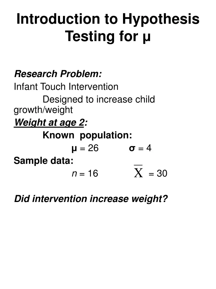
1. Introduction to HypothesisTesting for μ • Research Problem: • Infant Touch Intervention • Designed to increase child growth/weight • Weight at age 2: • Known population: • μ = 26 σ = 4 • Sample data: • n = 16 = 30 • Did intervention increase weight?

2. Hypothesis Testing: • Using sample data to evaluate an hypothesis about a population parameter. • Usually in the context of a research study -------evaluate effect of a “treatment” • Compare to known μ • Can’t take difference at face value • Differences between and μ expected simply on the basis of chance • sampling variability • How do we know if it’s just chance? • Sampling distributions!

3. Research Problem: • Infant Touch Intervention • Known population: μ = 26 σ = 4 • Assume intervention does NOT affect weight • Sample means ( ) should be close to population μ

6. Compare Sample Data to know population: • z-test = • How much does deviate from μ? • What is the probability of this occurrence? • How do we determine this probability?

7. Distribution of Sample Means (DSM)! • in the tails are low probability • How do we judge “low” probability of occurrence? • Widely accepted convention..... • < 5 in a 100 p< .05

8. Logic of Hypothesis Testing • Rules for deciding how to decide! • Easier to prove something is false • Assume opposite of what you believe… • try to discredit this assumption…. • Two competing hypotheses: • (1)Null Hypothesis (H0 ) • The one you assume is true • The one you hope to discredit • (2)Alternative Hypothesis (H1 ) • The one you think is true

9. Inferential statistics: • Procedures revolve around H0 • Rules for deciding when to reject or retain H0 • Test statistics or significance tests: • Many types: z-test t-test F-test • Depends on type of data and research design • Based on sampling distributions, assumes H0 is true • If observed statistic is improbable given H0, then H0 is rejected

10. Hypothesis Testing Steps: • (1)State the Research Problem • Derived from theory • example: • Does touch increase child growth/weight? • (2)State statistical hypotheses • Two contradictory hypotheses: • (a) Null Hypothesis: H0 • There is noeffect • (b) Scientific Hypothesis: H1 • There is an effect • Also called alternative hypothesis

11. Form of Ho and H1 for one-sample mean: • H0 : μ = 26 • H1 : μ <> 26 • Always about a population parameter, not a statistic • H0 : μ = population value • H1 : μ <> population value • non-directional (two-tailed) hypothesis • mutually exclusive :cannot both be true

12. Example: • Infant Touch Intervention • Known population:μ = 26 σ = 4 • Did intervention affect child weight? • Statistical Hypotheses: • H0: μ = 26 • H1 : μ <> 26

13. Hypothesis Testing Steps: • (3)Create decision rule • Decision rule revolves around H0, notH1 • When will you reject Ho? • …when values of are unlikely given H0 • Look in tails of sampling distribution • Divide distribution into two parts: • Values that are likely if H0 is true • Values close to H0 • Values that are very unlikely if H0 is true • Values far from H0 • Values in the tails • How do we decide what is likely and unlikely?

15. Level of significance = alpha level = α • Probability chosen as criteria for “unlikely” • Common convention: α = .05 (5%) • Critical value = boundary between likely/unlikely outcomes • Critical region = area beyond the critical value

16. Decision rule: • Reject H0 when observed test-statistic (z) equals or exceeds the Critical Value (when z falls within the Critical Region) • Otherwise, Retain H0

17. Hypothesis Testing Steps: • (4) Collect data and Calculate “observed” test statistic • z-test for one sample mean: • A closer look at z: • z = sample mean – hypothesized population μ • standard error • z = observed difference • difference due to chance

18. Hypothesis Testing Steps: • (5)Make a decision • Two possible decisions: • Reject H0 • Retain (Fail to Reject) H0 • Does observed z equal or exceed CV? • (Does it fall in the critical region?) • If YES, • Reject H0 = “statistically significant” finding • If NO, • Fail to Reject H0 = “non-significant” finding

19. Hypothesis Testing Steps: • (6)Interpret results • Return to research question • statistical significance = not likely to be due to chance • Never “prove” or H0 or H1

20. Example • (1) Does touch increase weight? • Population: μ = 26 σ = 4 • (2) Statistical Hypotheses: • H0 : μ = • H1 : μ <> • (3) Decision Rule: • α = .05 • Critical value: • (4) Collect sample data: n = 16 = 30 • Compute z-statistic: • (5) Make a decision: • (6) Interpret results: • Intervention appears to increase weight. Difference not likely to be due to chance.

21. More about alpha (α) levels: • most common : α = .05 • more stringent : α = .01 • α = .001 • Critical values for two-tailed z-test:

23.  = .05 p=.025 p=.025 1.96 +1.96 More About Hypothesis Testing • I. Two-tailed vs. One-tailed hypotheses • A. Two-tailed (non-directional): • H0:  = 26 • H1 :  26 • Region of rejection in both tails: • Divide α in half: • probability in each tail = α / 2

24. p=.05 z +1.65 p=.05 z 1.65 • B. One-tailed (directional): • H0:  26 • H1 :  > 26 • Upper tail critical: • H0 :  26 • H1 :  < 26 • Lower tail critical:

25. Examples: • Research hypotheses regarding IQ, where hyp= 100 • (1)Living next to a power station will lower IQ? • H0: • H1: • (2)Living next to a power station will increase IQ? • H0: • H1: • (3) Living next to a power station will affect IQ? • H0: • H1: • When in doubt, choose two-tailed!

26. II. Selecting a critical value • Will be based on two pieces of information: • (a) Desired level of significance (α)? • α = alpha level • .05 .01 .001 • (b)Is H0 one-tailed or two-tailed? • If one-tailed: find CV for α • CV will be either + or - • If two-tailed: find CV for α /2 • CV will be both +/ - • Most Common choices: • α = .05 • two-tailed test

27. Commonly used Critical Values for the z-statistic • Hypothesis α = .05 α =.01 • ______________________________________________ • Two-tailed  1.96  2.58 • H0:  = x • H1:  x • One-tailed upper + 1.65 + 2.33 • H0:  x • H1:  > x • One-tailed lower  1.65  2.33 • H0:  x • H1:  < x • ______________________________________________ • Where x = any hypothesized value of  under H0 • Note: critical values are larger when: • a more stringent (.01 vs. .05) • test is two-tailed vs. one-tailed

28. III. Outcomes of Hypothesis Testing • Four possible outcomes: • True status of H0 • No Effect Effect • H0 true H0 false • Reject H0 • Decision • Retain H0 • Type I Error:Rejecting H0 when it’s actually true • Type II Error:Retaining H0 when it’s actually false • We never know the “truth” • Try to minimize probability of making a mistake

29. A. Assume Ho is true • Only one mistake is relevant Type I error • α= level of significance • p (Type I error) • 1- α = level of confidence • p(correct decision), when H0 true • if α = .05, confidence = .95 • if α = .01, confidence = .99 • So, mistakes will be rare when H0 is true! • How do we minimize Type I error? • WE control error by choosing level of significance (α) • Choose α = .01 or .001 if error would be very serious • Otherwise, α = .05 is small but reasonable risk

30. B. Assume Ho is false • Only one mistake is relevant Type II error •  = probability of Type II error • 1- = ”Power” • p(correct decision), when H0 false • How big is the “treatment effect”? • When “effect size” is big: • Effect is easy to detect •  is small (power is high) • When “effect size” is small: • Effect is easy to “miss” •  is large (power is low)

31. How do you determine  and power (1-) • No single value for any hypothesis test • Requires us to guess how big the “effect” is • Power = probability of making a correct decision • when H0 is FALSE • C. How do we increase POWER? • Power will be greater (and Type II error smaller): • Larger sample size (n)Single best way to increase power! • Larger treatment effect • Less stringent a level e.g., choose .05 vs. .01 • One-tailed vs. two-tailed tests

32. a 1-  Type I Error Power 1-a Confidence Type II Error Four Possible Outcomes of an Hypothesis Test • True status of H0 • H0 true H0 false • Reject H0 • Decision • Retain H0 • α = level of significance • probability of Type I Error • risk of rejecting a true H0 • 1- α = level of confidence • p (making correct decision), if H0 true •  = probability of Type II Error • risk of retaining a false H0 • 1- = power • p(making correct decision), if H0 false • ability to detect true effect

33. IV. Additional Comments • A. Statistical significance vs. practical significance • “Statistically Significant” = H0 rejected • B. Assumptions of the z-test (see book for review): • DSM is normal • Known  (and  unaffected by treatment) • Random sampling • Independent observations • Rare to actually know ! • Preview  use t statistic when  unknown

34. V. Reporting Results of an Hypothesis Test • If you reject H0: • “There was a statistically significantdifference in weight between children in the intervention sample (M = 30 lbs) and the general population (M = 30 lbs),z = 4.0, p < .05, two-tailed.” • If you fail to reject H0 : • “There was nosignificantdifference in weight between children in the intervention sample (M = 30 lbs) and the general population (M = 30 lbs),z = 1.0, p > .05, two-tailed.”

35. A closer look… • z = 4.0, p < .05 test statistic level of significance observed value

36. VI. Effect Size • Statistical significance vs. practical importance • How large is the effect, in practical terms? • Effect size = descriptive statistics that indicate the magnitude of an effect • Cohen’s d • Difference between means in standard deviation units • Guidelines for interpreting Cohen’s d