Download
1 / 14
140 likes | 252 Views
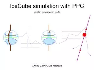
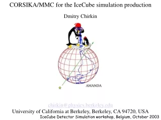
IceCube simulation with PPC. Dmitry Chirkin, UW Madison, 2010. Photonics. First, run photonics to fill space with photons, tabulate the result Create such tables for nominal light sources: cascade and uniform half-muon

E N D
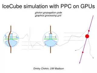
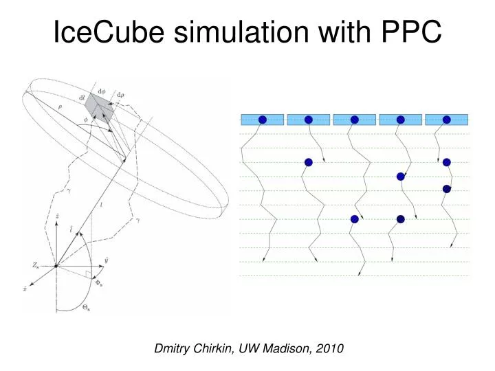
IceCube simulation with PPC Dmitry Chirkin, UW Madison, 2010
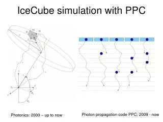
Photonics • First, run photonics to fill space with photons, tabulate the result • Create such tables for nominal light sources: cascade and uniform half-muon • Simulate photon propagation by looking up photon density in tabulated distributions • Table generation is slow • Simulation suffers from a wide range of binning artifacts • Simulation is also slow! (most time is spent loading the tables)
Direct photon tracking with PPC photon propagation code • simulating flasher/standard candle photons • same code for muon/cascade simulation • using Henyey-Greenstein scattering function with <cos q>=0.8 • using tabulated (in 10 m depth slices) layered ice structure • employing 6-parameter ice model to extrapolate in wavelength • transparent folding of acceptance and efficiencies • precise tracking through layers of ice, no interpolation needed • much faster than photonics for E-2 nugen and unweighted CORSIKA: • 1000-1200 corsika files (4 sec each) in 24 hours • 2500-3500 E-2 nugen files in 24 hours IC-40 i.e., 10000 E-2 nugen files in ~3-4 days on 6-GPU cudatest in ~1 day on 3 cuda00X computers
PPC simulation on GPU graphics processing unit execution threads propagation steps (between scatterings) photon absorbed new photon created (taken from the pool) threads complete their execution (no more photons) Running on an NVidia GTX 295 CUDA-capable card, ppc is configured with: 384 threads in 33 blocks (total of 12672 threads) average of ~ 512 photons per thread (total of 6.5 . 106 photons per call)
Photon Propagation Code: PPC • There are 5 versions of the ppc: • original c++ • "fast" c++ • in Assembly • for CUDA GPU • icetray module All versions verified to produce identical results comparison with i3mcml http://icecube.wisc.edu/~dima/work/WISC/ppc/
cudatest 1 x ASUS P6T Motherboard 12 GB Ram 1 x Intel i7 920 (2.66 GHz) 1 x NZXT Tempest case 1.5 TB Hard Drive 1 x OEM Samsung SH-S223B/BEBE DVDRW Drive 1 x Microsoft Business Hardware Pack Keyboard and Mouse Combo 1 x Acer H233Hbmid 23" Widescreen HD LCD Monitor 1 x EVGA GeForce GTX295 CoOp Edition 2 x EVGA GeForce GTX295 Superclocked Edition 1 x Corsair CMPSU-1000HX 1000W ATX12V 2.2 power supply 1 x FSP Group Booster X5 450W supplementary power supply 3 GTX295 (=6 GPUs and a total of 1440 cores). NVidia claims a total of 5.36 Teraflops. In total we have spent $3215.48 for the system including monitor and a first power supply which we had to replace later. Update (3/5/10): all 3 GTX295 cards are now Superclocked Edition
Ice Fitting with PPC • It became obvious that the AHA ice parameterization is inaccurate in explaining the IceCube data (flasher, standard candles, muon background, atmospheric neutrino, more?) and a new direct fitting procedure was implemented: • For each set of ice parameters (scattering and absorption at ~100 depths (10-meter slices in depth) the detector response was simulated to 60 different flasher events (on string 63). This response was compared to the data with a likelihood function, which took into account both statistical and 10% belt of systematic errors. • The minimum found with AHA as the initial approximation resulted in SPICE(South Pole Ice) model • The minimum found with bulk ice as the initial approximation but combined with the dust logger data to extrapolate in x and y for positions other than that of string 63, and in depth above and below the detector, resulted in SPICE2(South Pole Ice, second iteration) model • More iterations may be possible to take into account other sources of data
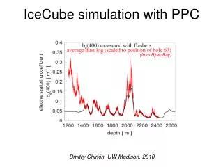
Correlation with dust logger data (from Ryan Bay) effective scattering coefficient Scaling to the location of hole 50 fitted detector region Ice tilt as measured by the dust loggers was easily implemented. This was not possible with photonics.
Rapid improvements in simulation by Anne Schukraft by Sean Grullon Downward-going CORSIKA simulation Up-going muon neutrino simulation
Summary • PPC is a direct photon propagation tool: • extensively verified • uncompromising precision of ice description • no interpolation • uses full xy map of ice properties • reached the production level of performance • PPC-GPU allowed to develop the SPICE2 (South Pole ICE) model: • fitted to IceCube flasher data collected on string 63 in 2008 • demonstrated remarkable correlation with the dust logger data • therefore was extended to incorporate these data • use of flasher timing information is possible (SPICE2+) • Rapid progress in simulation leads to very good agreement with data: • In-situ flasher simulation • background muon simulation • neutrino simulation
SPICE verification with CORSIKAby Anne Schukraft Already much better agreement than with AHA! Some disagreement remains, more work is needed
SPICE simulation of nmby Sean Grullon At the horizon: no need for exotic neutrino interaction ideas