Download
1 / 30
300 likes | 511 Views
Chapter 10. Risk Return & The Capital Asset Pricing Model (CAPM). To make “good” (i.e., value-maximizing) financial decisions, one must understands the relationship between risk and return We accept the notion that investors like returns and dislike risk

E N D
Chapter 10 Risk Return & The Capital Asset Pricing Model (CAPM) • To make “good” (i.e., value-maximizing) financial decisions, one must understands the relationship between risk and return • We accept the notion that investors like returns and dislike risk • Consider the following proxies for return and risk: Expected return- weighted average of the distribution of possible returns in the future. Variance of returns- a measure of the dispersion of the distribution of possible returns in the future. Jacoby, Stangeland and Wajeeh, 2000
Expected (Ex Ante) Return where, Rk = the return in state k (there are S states) Pk = the probability of return k (state k) An Example Consider the following return figures for the following year on stock XYZ under three alternative states of the economy PkRk Probability Return inState of Economy of state k state k +1% change in GNP 0.25 -5% +2% change in GNP 0.50 15% +3% change in GNP 0.25 35% 1.00
Expected Returns - An Example Q. Calculate the expected return on stock XYZ for the next year A. Use the following table PiRi PiRi Probability Return inState of Economy of state i state i State 1: +1% change in GNP 0.25 -5% State 2: +2% change in GNP 0.50 15% State 3: +3% change in GNP 0.25 35% Expected Return = Or, use the formula:
Variance and Standard Deviation of Returns where, Rk = the return in state k (there are S states) Pk = the probability of return k (state k) and s = the standard deviation of the return: An Example Recall the return figures for the following year on stock XYZ under three alternative states of the economy PkRk Probability Return inState of Economy of state k state k State 1: +1% change in GNP 0.25 -5% State 2: +2% change in GNP 0.50 15% State 3: +3% change in GNP 0.25 35% Expected Return = 15.00%
Variance & Standard Deviation - An Example Q. Calculate the variance of and standard deviation of returnson stock XYZ A. Use the following table State of Economy Pk X(Rk - E[R])2 = Pk(Rk - E[R])2 +1% change in GNP 0.25 0.04 +2% change in GNP 0.50 0.00 +3% change in GNP 0.25 0.04 Variance of Return =0.02 Or, use the formula: = Standard deviation:
Portfolio Return and Risk Q. Calculate the expected return on assets A and B for the next year, given the following distribution of returns: A. Expected returns E(RA) = (0.40%0.30) + (0.60%(-0.10)) = 0.06 = 6% E(RB) = (0.40%(-0.05)) + (0.60%0.25) = 0.13 = 13% State of the Probability Return on Return oneconomy of state asset A asset B Boom 0.40 30% -5% Bust 0.60 -10% 25% Jacoby, Stangeland and Wajeeh, 2000
Q. Calculate the variance of the above assets A and B A. Variances Var(RA) = 0.40%(0.30 - 0.06)2 + 0.60%(-0.10 - 0.06)2 = 0.0384 Var(RB) = 0.40%(-0.05 - 0.13)2 + 0.60%(0.25 - 0.13)2 = 0.0216 Q. Calculate the standard deviations of the above assets A and B A. Standard Deviations sA = (0.0384)1/2 = 0.196 = 19.6% sB = (0.0216)1/2 = 0.147 = 14.7% Jacoby, Stangeland and Wajeeh, 2000
Returns and Risk for Portfolios - 2 Assets Expected Return on a Portfolio The Expected Return on Portfolio p with N securities where, E[Ri]= expected return of security i Xi = proportion of portfolio's initial value invested in security i Example - Consider a portfolio p with 2 assets: 50% invested in asset A and 50% invested in asset B. The Portfolio expected return is given by: E(RP) = XAE(RA) + XBE(RB) =
Variance of a Portfolio The variance of portfolio p with two assets (A and B) where, Standard Deviation of a Portfolio The standard deviation of portfolio p with two assets (A and B) Jacoby, Stangeland and Wajeeh, 2000
Q. Calculate the variance of portfolio p (50% in A and 50% in B) A. Recall:Var(RA) = 0.0384, and Var(RB) = 0.0216 First, we need to calculate the covariance b/w A and B: The variance of portfolio p Q. Calculate the standard deviations of portfolio p A. Standard Deviations sp = (0.0006)1/2 = 0.0245 = 2.45%
The Effect of Diversification on Portfolio Risk Note: • E(RP) = XAE(RA) + XBE(RB) = 9.5%, but • Var(Rp) =0.0006 <XAVar(RA) + XBVar(RB) = (0.50% 0.0384) + (0.50%0.0216) = 0.03 • This means that by combining assets A and B into portfolio p, we eliminate some risk (mainly due to the covariance term) • Diversification - Strategy designed to reduce risk by spreading the portfolio across many investments • Two types of Risk: Unsystematic/unique/asset-specific risks - can be diversified away Systematic or “market” risks - can’t be diversified away • In general, a well diversified portfolio can be created by randomly combining 25 risky securities into a portfolio (with little (no) cost).
Portfolio Diversification Average annualstandard deviation (%) 49.2 Diversifiable (nonsystematic) risk 23.9 19.2 Nondiversifiable(systematic) risk Number of stocksin portfolio 1 10 20 30 40 1000 Jacoby, Stangeland and Wajeeh, 2000
Beta and Unique Risk • Total risk = diversifiable risk + market risk • We assume that diversification is costless, thus diversifiable (nonsystematic) risk is irrelevant • Investors should only care about nondiversifiable (systematic) market risk • Market risk is measured by beta - the sensitivity to market changes • Example: Return (%) State of the economy TSE300 BCE Good 18 26 Poor 6 -4 Jacoby, Stangeland and Wajeeh, 2000
Beta and Market Risk Interpretation: Following a change of +1% (-1%) in the market return, the return on BCE will change by +2.5% (-2.5%) NOTE: If the security has a -ve cov w/ TSE 300 => The Characteristic Line • (18%, 26%) • (6%, -4%)
Beta and Unique Risk • Market Portfolio - Portfolio of all assets in the economy. In practice a broad stock market index, such as the TSE300, is used to represent the market • Beta (b )- Sensitivity of a stock’s return to the return on the market portfolio Covariance of security i’s return with the market return Variance of market return Jacoby, Stangeland and Wajeeh, 2000
Markowitz Portfolio Theory • We saw that combining stocks into portfolios can reduce standard deviation • Covariance, or the correlation coefficient, make this possible: The standard deviation of portfolio p (with XA in A and XB in B): Note: , or Thus, Jacoby, Stangeland and Wajeeh, 2000
Markowitz Portfolio Theory - An Example • Consider assets Y and Z, with • Consider portfolio p consisting of both Y and Z. Then, we have: Expected Return of p Standard Deviation of p Jacoby, Stangeland and Wajeeh, 2000
Look at the next 3 cases (for the correlation coefficient): • Where
The Shape of the Markowitz Frontier - An Example . r = -1 Y r = 0 . Z r = +1 Jacoby, Stangeland and Wajeeh, 2000
Efficient Sets and Diversification r = -1 r < 1 -1 < r = 1 Jacoby, Stangeland and Wajeeh, 2000
The Efficient (Markowitz) FrontierThe 2-Asset Case • Expected Returns and Standard Deviations vary given different weighted combinations of the two stocks • The Feasible Set is on the curve Z-Y • The Efficient Set is on the MV-Y segment only Expected Return (%) Stock Y Minimum Variance Portfolio (MV) 75% in Z and 25% in Y MV Stock Z Standard Deviation
U MV The Efficient (Markowitz) FrontierThe Multi-Asset Case • Each half egg shell represents the possible weighted combinations for two assets • The Feasible Set is onand inside the envelope curve • The composite of all asset sets (envelope), and in particular the segment MV-U constitutes the efficient frontier Expected Return (%) Minimum Variance Portfolio (MV) Standard Deviation
Efficient Frontier • We assume that investors are rational (prefer more to less) and risk averse Goal is to move UP and LEFT. WHY? Expected Return (%) Standard Deviation (Risk) Jacoby, Stangeland and Wajeeh, 2000
Which Asset Dominates? Expected Return (%) Low Risk High Return High Risk High Return Low Risk Low Return High Risk Low Return Standard Deviation (Risk) Jacoby, Stangeland and Wajeeh, 2000
Short Selling • Definition The sale of a security that the investor does not own • How? Borrow the security from your broker and sell it in the open market • Cash Flow At the initiation of the short sell, your only cash flow, is the proceeds from selling the security • Closing the Short Eventually you will have to buy the security back in order to return it to the broker • Cash Flow At the elimination of the short sell, your only cash flow, is the price you have to pay for the security in the open market Jacoby, Stangeland and Wajeeh, 2000
Short Selling A Treasury Bill - An Example • The Security • A Treasury bill is a zero-coupon bond issued by the Government, with a face value of $100, and with a maturity no longer than one year • If the yield on a 1-year T-bill is 5%, then its current price is: 100/1.051 = $95.24 • The Short sell Borrow the 1-year T-bill from your broker and sell it in the open market $95.24 • Cash Flow The short sell proceeds: $95.24 • Closing the Short At the end of the year - buy the T-bill back (an instant before it matures) in order to return it to the broker • Cash Flow The price you have to pay for the T-bill in the open market an instant before maturity (in 1 year): 100/1.050 = $100 • Risk-Free Borrowing This transaction is equivalent to borrowing $95.24 for one year, and paying back $ 100 in a year. The interest rate is: (100/95.24) -1 = 5% = the 1-year T-bill yield
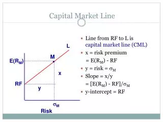
The Capital Market Line (CML)The Efficient Frontier With Risk-Free Borrowing and Lending • Lending or Borrowing at the risk free rate (Rf) allows us to exist outside the • Markowitz frontier. • We can create portfolio A by investing in both Rf (lending money) and M • We can create portfolio B by short selling Rf (borrowing money) and holding M . Expected returnof portfolio CML CML is the new efficient frontier B . M . A Risk-freerate (Rf ) Standarddeviation ofportfolio’s return.
The Capital Asset Pricing Model (CAPM) Note • all securities are in M, and • all investors have M in their portfolios since they are all on the new efficient frontier - CML - investing in Rf and M. Therefore Investors are only concerned with and , and with the contribution of each security i to M, in terms of • contribution of systematic risk (measured by beta) • contribution of expected return According to the CAPM: where,
The Security Market Line (SML) The Capital Asset Pricing Model (SML): Note: (1) -> entire risk of i is diversified away in M (2) -> security i contributes the average risk of M SML . M 1
The Security Market Line (SML) • The SML is always linear • CML - just for efficient portfolios SML - for any securityand portfolio (efficient or inefficient) Example: Consider stocks A and B, with: ba = 0.8,bb = 1.2, let E[Rm] = 14% and Rf = 4%. By the SML: E[Ra] = E[Rb] = Consider a portfolio p, with 60% invested in A and 40% invested in B, then: E[Rp] = XaE[Ra] + XbE[Rb] = 0.6$12% + 0.4$16% = 13.6%, and bp = Xa ba + Xb bb = 0.6$0.8 + 0.4$1.2 = 0.96 By the CAPM: E[Rp] = 4% + 0.96[14% - 4%] = 13.6% * If A and B are on the SML => P is also on SML