PHONOLOGY and the art of Automatic Speech Recognition

1. PHONOLOGYand the art ofAutomatic Speech Recognition Mark Hasegawa-Johnson ECE Department and the Beckman Institute for Advanced Science and Technology University of Illinois Urbana-Champaign, Illinois, USA

2. Outline • A Brief History of Ideas • The Prosodic Hierarchy • The Utterance • End-of-Turn Detection • The Intonational Phrase • Prosody-Dependent Speech Recognition • The Word • Articulatory Phonology Models of Coarticulation • The Syllable • Landmark-Based Speech Recognition • Audiovisual Speech Recognition • Analysis • Integration: Current Research Directions

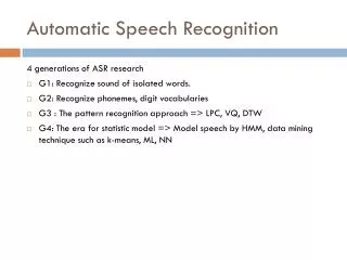
3. A Brief History of Ideas: Global • Mechanics • Science: 1687 (Newton’s Principia) • Technology: 1825 (Stockton & Darlington Railroad opens) • Human Benefits: 1850 (World per capita GDP, $800 in 2005 dollars, annual growth rate rises to 1%) • Electricity and Magnetism • Science: 1745 (van Muschenbroek invents Leyden jar) • Technology: 1876 (Bell invents telephone) • Human Benefits: 1950 (World per capita GDP, $2100, annual growth rate rises to 3%) • Spoken Communication • Science: 1867 (Bell proposes “Universal Alphabetic,” drawing on Panini, Tang Dynasty, King Sejong, Leibniz, Duponceau) • Technology: 1978 (TI sells the “Speak and Spell”) • Human Benefits: 2045 (language-independent markets for capital and intellectual talent drive the world per capita GDP, $30000, to a growth rate above 4% annually)

4. A Brief History of Ideas: Local • The Prosodic Hierarchy • Based on ideas of Selkirk, 1981; Nespor and Vogel, 1986 • End-of-Turn Detection • Reported research was performed by Kyle Gorman advised by Cole, Fleck, and Hasegawa-Johnson • Prosody-Dependent Speech Recognition • Based on ideas of Ostendorf, Byrne, Shriberg, Talkin, Waibel et al., 1996 • Reported research was performed by Ken Chen, Sarah Borys, and Sung-Suk Kim advised by Cole and Hasegawa-Johnson • Pronunciation Modeling based on Articulatory Phonology • Collaboration with Karen Livescu, creator of the Articulatory Feature model • Landmark-Based Speech Recognition • Based on ideas of Stevens, Manuel, Shattuck-Hufnagel, and Liu, 1992 • Reported research was performed by Sarah Borys, Amit Juneja and Karen Livescu advised by Niyogi, Glass, Espy-Wilson, and Hasegawa-Johnson • Audiovisual Speech Recognition • Based on the algorithms of Chu and Huang, 2001 • Reported research was performed by Ming Liu, Kate Saenko, Partha Lal, Mark Hasegawa-Johnson, Karen Livescu, Özgur Çetin

5. The Prosodic Hierarchy • Layered Constituents: Ci can only dominate Ck for k > i • Headed Constituents: Each Ci dominates at least one Ck • Non-Recursive Layering: No Ci dominates a Ci • Exhaustive Layering: No Ci dominates a Ci+2

6. Prosody: The Units of Articulatory Planning and Perception • Processes bounded within theUtterance • turn-taking cues, e.g., pause, duration, pitch, lexical cues • Processes bounded within theIntonational Phrase • sequencing/stair-stepping of pitch accents • phrase-final pitch effects: declarative fall, question rise, … • Processes bounded within theIntermediate Phrase • phrasal stress/ pitch accent • phrase tone • Processes bounded within theProsodic Word • co-articulation • Processes bounded within theFoot • vowel reduction, lexical stress • Processes bounded within theSyllable • abrupt onset, syllabic nuclear peak, abrupt offset

7. The Utterance

8. End-of-Turn Detection≠ Pause Detection(Local, Kelly and Wells, 1986)

9. Prosodic Features on Utterance-Final Word Can be Automatically Detected(Ferrer, Shriberg and Stolcke, 2002-3) Final word longer than a typical production of “oven” “Declaration fall:” pitch falls on utterance-final word “fire” has increased duration suggesting a possible EOT, but… “it” is very short, and ends abruptly with glottal stop.

10. Prosodic Features for EOT Detection(Gorman, Cole, Hasegawa-Johnson and Fleck, LSA 2007) • Pause Features: • Silence • Instant-response classifiers: truncate above pauses after 80, 100, …, 300ms, results are stable with pause duration truncated at 300ms • Duration Features: • Normalized last stressed vowel duration • Last stressed rhyme duration • Last rhyme duration • Pitch Features: • Minimum or median, last word or last N frames • F0 slope of word (continuous), or at boundary (categorical) • Context Features: • Speaker gender • Number of words since turn beginning • Length of previous pause

11. Prosodic Features for EOT Detection(Gorman, Cole, Hasegawa-Johnson and Fleck, LSA 2007)

12. The Intonational Phrase

13. Intonational Phrases and Pitch Accents • Tagged Transcription: Wanted*B4 chief* justice* of the Massachusetts* supreme court*B4 • B4 denotes intonational-phrase-final word • * denotes pitch accented word • Data: Boston Radio Speech corpus • 7 talkers; Professional radio announcers • About 3.5 hours of speech prosodically transcribed (ToBI = “tones and break indices” notation) • Largest prosodically transcribed English database, but… • Less than 1% of size of speech recognition training databases: e.g., too small to train triphones

14. Intonational Phrases and Pitch Accents: a Bayesian Network Model of Speech(Chen, Hasegawa-Johnson et al., 2003) Hidden Random Variables: W: words S: syntactic tags (POS, phrase) P: prosodic tags (phrse, accent) I: index of phone within word Q: phones H: phone-level prosodic tags T: transition (word, phone, none) Observed Variables: X: acoustic-phonetic features Y: acoustic-prosodic features S Word-Level Tags W P I Q H Phone-Level Tags T X Y Acoustic Features

15. Intonational Phrases and Pitch Accents: Prosody-Dependent Speech Recognition W* = argmaxW maxP,S,Q,H p(W,P,S) X p(Q,H|W,P) X p(X,Y|Q,H) p(Q,H|W,P): “Pronunciation Model” Specifies the phones used to pronounce word W in context P p(X,Y|Q,H): “Acoustic Model” Specifies the acoustic signal that implements phones Q in context H p(W,P,S): “Language Model” Specifies the probability of word string W jointly with syntax/prosody tags S,P W,P,S Q,H X,Y

16. Pronunciation Model: p(Q,H|W,P) • Tagged Transcription: Wanted*B4 chief* justice* of the Massachusetts* supreme court*B4 • Lexicon: • Each word has four entries • wanted, wanted*, wantedB4, wanted*B4 • IP boundary applies to phones in rhyme of final syllable • wantedB4w ɑ n təB4 dB4 • Accent applies to phones in lexically stressed syllable • wanted*w* ɑ* n*t ə d

17. Acoustic Model: p(X,Y|Q,H) In order to train on such a small database, we propose a Factored Acoustic Model: p(X,Y|Q,A,B) = Pi ∈{1,…,L} p(di|qi,bi) Pt ∈{1,…,di} p(xt|qi) p(yt|qi,ai) Hidden Variables, Phone-Synchronous: • prosody-independent phone label qi ∈ {ɑ,ə,t,d,…} • pitch accent type ai∈ {Accented,Unaccented} • intonational phrase position bi∈ {Final,Nonfinal} • di = duration of phone qi Observed Variables, Frame-Synchronous: • xt = acoustic-phonetic features (MFCC or PLP) • yt = acoustic-prosodic features (accent detector)

18. Acoustic-Prosodic Observations: yt = ANN(lnf0(t-5),…,lnf0(t+5)) TDRNN = time-delay neural network (Kim, Hasegawa-Johnson and Chen, 2003): a nonlinear dynamic system trained to estimate degree of phrasal prominence (pink) given F0 and energy (F0=blue)

19. Explicit Duration HMM: Phrase-Final vs. Non-Final Duration Histograms /ɑ/ phrase-medial and phrase-final /ɕ/ phrase-medial and phrase-final

20. A Factored Language Model Prosodically tagged words: cats* climb trees*% • Unfactored: Prosody and word string jointly modeled: p( trees*% | cats* climb ) • Factored: • Prosody depends on syntax: p( w*% | N V N, w* w ) • Syntax depends on words: p( N V N | cats climb trees ) Unfactored pi-1,wi-1 pi,wi Factored pi-1 pi wi-1 wi si-1 si

21. Result: Syntactic Mediation of Prosody Reduces Perplexity and WER Factored Model: Reduces Perplexity by 35% Reduces WER by 4% Syntactic Tags: For pitch accent: • POS sufficient For IP boundary: • Parse information useful if available pi-1 pi wi-1 wi si-1 si

22. Syntactic Factors: POS, Syntactic Phrase Boundary Depth

23. Results: Word Error Rate (Boston Radio Speech Corpus)

24. The Word

25. Pronunciation Variability in Spontaneous Speech • Reduction processes take place within a prosodic word, but.. • Prosodic word = one or two lexical words, e.g., • “like a” = /laja/ • “of them” = /əvəm/ • “Like a ton of them were on, like, …” • laja tã əvəm wɚ ɔn, lajk…

26. Coarticulation: the Gestural Phonology Model(Browman and Goldstein, 1992) Canonical Pronunciation Overlapped Gestures “everybody” “erwodi” Lip Gestures (Phonological Planning Units) Lip Aperture Tract Variable (Articulatory Planning Unit) Motor Neural Commands to the Lips /v/ /r/ /i/ /b/ /ʌ/ /i/ /v/ /b/ /r/ /i/ /ʌ/ /i/ Lip Opening Lip Opening Time (Mental Clock Units) Time (Mental Clock Units)

27. Working hypothesis: prosodic word boundaries block gestural overlap Coarticulation: the Gestural Phonology Model(Browman and Goldstein, 1992) “everybody” → “erwodi” /v/ /b/ Lips /r/ /ʌ/ /i/ /r/ /d/ Tongue /ɛ/ /i/ /v/ /b/ /d/ Glottis /ɛ/ /r/ /ʌ/ /i/ time

28. Simplified Gestural Phonology: Coarticulation = Lazy Articulators(Livescu and Glass, 2004)

29. Pronunciation Model: Dynamic Bayesian Network (DBN) with Partially Asynchronous Articulators(Livescu and Glass, 2004) • wordt: word ID at frame #t • wdTrt: word transition? • indti: which gesture, from • the canonical word model, • should articulator i be • trying to implement? • asyncti;j: how asynchronous • are articulators i and j? • Uti: canonical setting of • articulator #i • Sti: surface setting of • articulator #i

30. Articulatory Feature DBN Experiments • Background: • [Livescu and Glass, 2004]: • AF model predicts mapping from canonical pronunciations to human transcriptions better than HMM • [Saenko and Livescu, 2006]: • AF model recognizes visible speech better than HMM • To be presented today: • AF model as part of a landmark-based speech recognizer: [Hasegawa-Johnson, …, Livescu, et al., WS04]: • AF model for audiovisual speech recognition: [Livescu, …, Hasegawa-Johnson, et al., WS06]

31. The Syllable: Landmark-Based Speech Recognition

32. What are Landmarks? • Instants of rapid spectral change (dX/dt). • Instants of high spectral entropy (H((X(t)|X(t-1))). • Instants of high mutual information between phoneme and signal (I(q;X(t-d),…,X(t+d)). Where do these things happen? • Consonant closures (fricative, stop, nasal) • Consonant releases (fricative, stop, nasal) • Syllable nuclei

33. Landmark-Based Speech Recognition MAP transcription: … backed up … Search Space: … … buck up … … big dope … … backed up … … bagged up … … … big doowop … … ONSET ONSET Syllable Structure NUCLEUS NUCLEUS CODA CODA

34. Stop Detection using Support Vector Machines(Niyogi, Ramesh, and Burges, 1999, 2002) False Acceptance vs. False Rejection Errors per 10ms frame, Four Types of Stop Detectors (1) Delta-Energy (“Deriv”): Equal Error Rate = 0.2% (2) HMM (*): False Rejection Error=0.3% (3) Linear SVM: EER = 0.15% (4) RBF SVM: Equal Error Rate=0.13%

35. Two Types of SVMs: Landmark Detectors (p(landmark(t)),Landmark Classifiers (p(place-features(t)|landmark(t)) 2000-dimensional acoustic feature vector SVM Discriminant yi(t) Sigmoid or Histogram Posterior probability of distinctive feature p(di(t)=1 | yi(t))

36. Acoustic Feature Vector: Local Cepstrogram,Formants, Auditory Modeling Features Covering +/-70ms

37. SVM Training: Accuracy, Per Frame, in Percent (Chance=50%)

38. SVM/HMM Hybrid(Borys and Hasegawa-Johnson, ICSLP 2005) • 10 landmark-detection SVMs • 23 landmark-classification SVMs • Acoustic features: MFCC+d+dd, formant freqs+amps • HMM baseline speech recognizer: 3 states per phone, constrained only by a phoneme bigram • Raw real-valued SVM discriminant output fed to HMM, modeled there using mixture Gaussian PDFs, as in the “tandem” NN/HMM hybrid (Ellis et al., 2000)

39. DBN-SVM Model of Pronunciation Variability(Hasegawa-Johnson, Baker, …, Livescu et al., WS04, ICASSP 2005) Word LIKE A Canonical Form … Tongue closed Tongue Mid Tongue front Tongue open … Surface Form Tongue front Semi-closed Tongue Front Tongue open … Manner Glide Front Vowel Place Palatal SVM Outputs p( gPGR(x) | palatal glide release) p( gGR(x) | glide release ) x: Multi-Frame Observation including Spectrum, Formants, & Auditory Model

40. SVM/DBN Hybrid: Design Decisions • SVM Applied: When should SVM supply place feats to the DBN? • Landmarks: Only at SVM-detected landmarks • Frames: In every frame • Use Place?: In frame-based hybrid, how use place features be used? • Always: use place features for segmentation and recognition • Recognition: use place features only for recognition • Selective: use only the high-accuracy place features; ignore others • Probs: How should SVM information be passed to the DBN? • Posterior: SVM output converted to a posterior probability • Likelihood: Posterior is normalized to estimate a pseudo-likelihood • DBN Training: How should DBN be trained? • Manual: Using manual landmark transcriptions (ICSI Switchboard) • SVMs: Using SVM-detected landmarks

41. Landmark-Based Speech Recognizer used to Rescore the 2003 SRI Decipher System(Hasegawa-Johnson, Baker,…, Livescu, et al., WS04, ICASSP 2005) For each word hypothesis generated by the SRI Decipher Speech Recognizer: • SVM probabilities computed during word hypothesis, input to DBN • DBN computes a score S  P(word | evidence) • Final edge score is a weighted interpolation of first-pass speech recognizer scores, together with the DBN score

42. The Syllable: Audiovisual Speech

43. Why Use Visual Information? • Visuals are unaffected by noise • Human listeners use visuals in quiet: • McGurk and MacDonald, 1976: listeners unable to hear a /b/ if see lips that stay open • Human listeners use visuals in noise: • Sumby and Pollack, 1954: visible talker improves intelligibility in noise • Callan et al., 1997: pre-motor cortex activates when listening to speech at low SNR

44. Two Audiovisual Corpora • AVICAR • Collected at University of Illinois • 100 talkers (largest free AVSR database?) • Read digits, digit strings, letters, sentences • Naturalistic & Variable Lighting: Moving Car • Naturalistic & Variable Noise: Wind, Cars, … • CUAVE • Collected at Clemson University • 35 talkers • Read digits & digit strings • Controlled Lighting: Studio w/Green Screen • Controlled Noise: Electrically Added

45. 8 Mics, Pre-amps, Wooden Baffle. Best Place= Sunvisor. 4 Cameras, Glare Shields, Adjustable Mounting Best Place= Dashboard AVICAR Recording Hardware(Lee, Hasegawa-Johnson et al., 2004) System is not permanently installed; mounting requires 10 minutes.

46. Video: Face & Lip Tracking

47. Visual-Only Recognition Results • Isolated Digits • Video Features: Normalized DCT of the lip image • Standard HMM speech recognizer, number of states per digit depends on number of phonemes • Speaker-independent training, speaker-adapted recognition • Recognition results (WER, percent) • AVICAR: about 80% WER • CUAVE: about 60% WER • For comparison, other results reported for isolated digit recognition using controlled lighting, e.g., Chu and Huang 2002: about 60% WER

48. CUAVE Experiments(Livescu, …, Lal, Hasegawa-Johnson et al., WS06) • 169 utterances used, 10 digits each • NOISEX speech babble added at various SNRs • Experimental setup • Training on clean data, number of Gaussians tuned on clean dev set • Audio/video weights tuned on noise-specific dev sets • Uniform (“zero-gram”) language model • Decoding constrained to 10-word utterances (avoids language model scale/penalty tuning) • Thanks to Amar Subramanya at UW for the video observations • Thanks to Kate Saenko at MIT for initial Baselines, audio observations

49. Audio-only DBN Speech Recognizer phone_index_audio phone_transition_audio phone_name_audio observation_audio

50. Video-only DBN Speech Recognizer phone_index_video Phone_transition_video Phone_name_video observation_video