Networking II: The Link and Network Layers

1. Networking II:The Link and Network Layers

2. Announcements • Prelim II will be Thursday, November 20th, in class • Homework 5 available later today, November 4th • Vote today

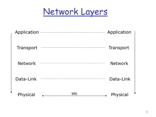
3. Review: OSI Levels • Physical Layer • electrical details of bits on the wire • Data Link Layer • sending “frames” of bits and error detection • Network Layer • routing packets to the destination • Transport Layer • reliable transmission of messages, disassembly/assembly, ordering, retransmission of lost packets • Session Layer • really part of transport, typically Not implemented • Presentation Layer • data representation in the message • Application • high-level protocols (mail, ftp, etc.)

4. Review: OSI Levels Node A Application Node B Application Presentation Presentation Session Session Transport Transport Network Network Data Link Data Link Physical Physical Network

5. What is purpose of this layer? • Invoke Physical Layer • Physically encode bits on the wire • Link = pipe to send information • E.g. point to point or broadcast • Can be built out of: • Twisted pair, coaxial cable, optical fiber, radio waves, etc • Links should only be able to send data • Could corrupt, lose, reorder, duplicate, (fail in other ways)

6. Header (Dest:2) Body (Data) Message ID:3 (sender) Broadcast Networks Details • Delivery: When you broadcast a packet, how does a receiver know who it is for? (packet goes to everyone!) • Put header on front of packet: [ Destination | Packet ] • Everyone gets packet, discards if not the target • In Ethernet, this check is done in hardware • No OS interrupt if not for particular destination • This is layering: we’re going to build complex network protocols by layering on top of the packet ID:1 (ignore) ID:4 (ignore) ID:2 (receive)

7. Switch Router Internet Point-to-point networks • Why have a shared broadcast medium? Why not simplify and only have point-to-point links + routers/switches? • Didn’t used to be cost-effective • Now, easy to make high-speed switches and routers that can forward packets from a sender to a receiver. • Point-to-point network: a network in which every physical wire is connected to only two computers • Switch: a bridge that transforms a shared-bus configuration into a point-to-point network. • Router: a device that acts as a junction between two networks to transfer data packets among them.

8. Point-to-Point Networks Discussion • Advantages: • Higher link performance • Can drive point-to-point link faster than broadcast link since less capacitance/less echoes (from impedance mismatches) • Greater aggregate bandwidth than broadcast link • Can have multiple senders at once • Can add capacity incrementally • Add more links/switches to get more capacity • Better fault tolerance (as in the Internet) • Lower Latency • No arbitration to send, although need buffer in the switch • Disadvantages: • More expensive than having everyone share broadcast link • However, technology costs now much cheaper • Examples • ATM (asynchronous transfer mode) • The first commercial point-to-point LAN • Inspiration taken from telephone network • Switched Ethernet • Same packet format and signaling as broadcast Ethernet, but only two machines on each ethernet.

9. How to connect routers/machines? • WAN/Router Connections • Commercial: • T1 (1.5 Mbps), T3 (44 Mbps) • OC1 (51 Mbps), OC3 (155 Mbps) • ISDN (64 Kbps) • Frame Relay (1-100 Mbps, usually 1.5 Mbps) • ATM (some Gbps) • To your home: • DSL • Cable • Local Area: • Ethernet: IEEE 802.3 (10 Mbps, 100 Mbps, 1 Gbps) • Wireless: IEEE 802.11 b/g/a (11 Mbps, 22 Mbps, 54 Mbps)

10. Link level Issues • Encoding: map bits to analog signals • Framing: Group bits into frames (packets) • Arbitration: multiple senders, one resource • Addressing: multiple receivers, one wire

11. Encoding • Map 1s and 0s to electric signals • Simple scheme: Non-Return to Zero (NRZ) • 0 = low voltage, 1 = high voltage • Problems: • How to tell an error? When jammed? When is bus idle? • When to sample? Clock recovery is difficult. • Idea: Recover clock using encoding transitions 1 0 1 1 0

12. 0 1 1 0 Manchester Encoding • Used by Ethernet • Idea: Map 0 to low-to-high transition, 1 to high-to-low • Plusses: can detect dead-link, can recover clock • Bad: reduce bandwidth, i.e. bit rate = ½ baud rate • If wire can do X transition per second?

13. Framing • Why send packets? • Error control • How do you know when to stop reading? • Sentinel approach: send start and end sequence • For example, if sentinel is 11111 • 11111 00101001111100 11111 10101001 11111 010011 11111 • What if sentinel appears in the data? • map sentinel to something else, receiver maps it back • Bit stuffing

14. Example: HDLC • High-Level Data Link Control (HLDC) • Data link layer protocol developed by the ISO • Same sentinel for begin and end: 0111 1110 • packet format: • Bit stuffing • Sender: If 5 1s then insert a 0 • Receiver: if 5 1s followed by a 0, remove 0 • Else read next bit • Packet size now depends on the contents 0111 1110 header data CRC 0111 1110 0111 1110 0111 1101 0 0111 1101 0 0111 1110

15. Broadcast Network Arbitration • Arbitration: Act of negotiating use of shared medium • What if two senders try to broadcast at same time? • Concurrent activity but can’t use shared memory to coordinate! • Aloha network (70’s): packet radio within Hawaii • Blind broadcast, with checksum at end of packet. If received correctly (not garbled), send back an acknowledgement. If not received correctly, discard. • Need checksum anyway – in case airplane flies overhead • Sender waits for a while, and if doesn’t get an acknowledgement, re-transmits. • If two senders try to send at same time, both get garbled, both simply re-send later. • Problem: Stability: what if load increases? • More collisions  less gets through more resent  more load…  More collisions… • Unfortunately: some sender may have started in clear, get scrambled without finishing

16. Arbitration • One medium, multiple senders • What did we do for CPU, memory, readers/writers? • New Problem: No centralized control • Approaches • TDMA: Time Division Multiple Access • Divide time into slots, round robin among senders • If you exceed the capacity  do not admit more (busy signal) • FDMA: Frequency Division Multiple Access (AMPS) • Divide spectrum into channels, give each sender a channel • If no more channels available, give a busy signal • Good for continuous streams: fixed delay, constant data rate • Bad for bursty Internet traffic: idle slots

17. Ethernet • Developed in 1976, Metcalfe and Boggs at Xerox • Uses CSMA/CD: • Carrier Sense Multiple Access with Collision Detection • Easy way to connect LANs Metcalfe’s Ethernet sketch

18. CSMA/CD • Carrier Sense: • Listen before you speak • Multiple Access: • Multiple hosts can access the network • Collision Detection: • Can make out if someone else started speaking Older Ethernet Frame

19. CSMA Wait until carrier free

20. CSMA/CD Garbled signals If the sender detects a collision, it will stop and then retry! What is the problem?

21. No Yes attempts < 16 attempts == 16 CSMA/CD Packet? Sense Carrier Detect Collision Send Discard Packet Jam channel b=CalcBackoff(); wait(b); attempts++;

22. Ethernet’s CSMA/CD (more) Jam Signal: make sure all other transmitters are aware of collision; 48 bits; Exponential Backoff: • Goal: adapt retransmission attempts to estimated current load • heavy load: random wait will be longer • Adaptive and Random • First time, pick random wait time with some initial mean. If collide again, pick random value from bigger mean wait time. Etc. • Randomness is important to decouple colliding senders • Scheme figures out how many people are trying to send! • Example • first collision: choose K from {0,1}; delay is K x 512 bit transmission times • after second collision: choose K from {0,1,2,3}… • after ten or more collisions, choose K from {0,1,2,3,4,…,1023}

23. Packet Size • If packets are too small, the collision goes unnoticed • Limit packet size • Limit network diameter • Use CRC to check frame integrity • truncated packets are filtered out

24. Ethernet Problems • What if there is a malicious user? • Might not use exponential backoff • Might listen promiscuously to packets • Integrating Fast and Gigabit Ethernet

25. Addressing & ARP • ARP is used to discover physical addresses • ARP = Address Resolution Protocol 128.84.96.89 128.84.96.90 128.84.96.91 “What is the physical address of the host named 128.84.96.89” “I’m at 1a:34:2c:9a:de:cc”

26. Addressing & RARP • RARP is used to discover virtual addresses • RARP = Reverse Address Resolution Protocol ??? 128.84.96.90 RARP Server 128.84.96.91 “I just got here. My physical address is 1a:34:2c:9a:de:cc. What’s my name ?” “Your name is 128.84.96.89”

27. Repeaters and Bridges • Both connect LAN segments • Usually do not originate data • Repeaters (Hubs): physical layer devices • forward packets on all LAN segments • Useful for increasing range • Increases contention • Bridges: link layer devices • Forward packets only if meant on that segment • Isolates congestion • More expensive

28. Backbone Bridge

29. Summary • Data Link Layer • layer two of the seven-layer OSI model • Layer two of the five-layer TCP/IP reference model as well. • Responds to service requests from the network layer and issues service requests to the physical layer. • Broadcast vs Point-to-point • Point-to-point is often higher performance, but traditionally higher cost as well • Switched Ethernet is common now • Data Link Layer Issues • Encoding: map bits to analog signals • Manchester encoding • Framing: Group bits into frames (packets) • Bit stuffing • Arbitration: multiple senders, one resource • Ethernet uses CSMA/CD (carrier sense multiple access/collision detection) • Addressing: multiple receivers, one wire • ARP (address resolution protocol)

30. The Network Layer

31. Review: OSI Levels • Physical Layer • electrical details of bits on the wire • Data Link Layer • sending “frames” of bits and error detection • Network Layer • routing packets to the destination • Transport Layer • reliable transmission of messages, disassembly/assembly, ordering, retransmission of lost packets • Session Layer • really part of transport, typically Not implemented • Presentation Layer • data representation in the message • Application • high-level protocols (mail, ftp, etc.)

32. Review: OSI Levels Node A Application Node B Application Presentation Presentation Session Session Transport Transport Network Network Data Link Data Link Physical Physical Network

33. Review: OSI Levels Node A Application Node B Application Presentation Presentation Session Session Transport Transport Router Network Network Network Data Link Data Link Data Link Physical Physical Physical Network

34. Given a packet, send it across the network to destination 2 key issues: Portability: connect different technologies Scalability To the Internet scale network data link physical network data link physical network data link physical network data link physical network data link physical network data link physical network data link physical network data link physical application transport network data link physical application transport network data link physical Purpose of Network layer

35. What does it involve? Two important functions: • routing: determine path from source to dest. • forwarding: move packets from router’s input to output T3 T1 T3 Sts-1 T1

36. Q: What service model for “channel” transporting packets from sender to receiver? guaranteed bandwidth? preservation of inter-packet timing (no jitter)? loss-free delivery? in-order delivery? congestion feedback to sender? Network service model ? ? ? The most important abstraction provided by network layer: service abstraction virtual circuit or datagram? Which things can be “faked” at the transport layer?

37. b b 1 1 B C B C A Two connection models • Connectionless (or “datagram”): • each packet contains enough information that routers can decide how to get it to its final destination • Connection-oriented (or “virtual circuit”) • first set up a connection between two nodes • label it (called a virtual circuit identifier (VCI)) • all packets carry label 1 A

38. used to setup, maintain teardown VC setup gives opportunity to reserve resources used in ATM (Asynchronous Transfer Mode), frame-relay, X.25 (or OSI protocol suite) not used in today’s Internet application transport network data link physical application transport network data link physical Virtual circuits: signaling protocols 6. Receive data 5. Data flow begins 4. Call connected 3. Accept call 1. Initiate call 2. incoming call

39. 2 1 5 1 2 2 1 a b c Virtual circuit switching • Forming a circuit: • send a connection request from A to B. • Contains VCI + address of B • VCI is the Virtual Circuit Identifier • rule: VCI must be unique on the link its used on • switch creates an entry mapping input messages with VCI to output port • switch picks a new VCI unique between it and next switch

40. a b c Virtual circuit forwarding • For each VCI switch has a table which maps input link to output link and gives the new VCI to use • if a’s messages come into switch 1 on link 2 and go out on link 3 then the table will be: (Input link,VCI) (output link, new VCI) (1, 2) (?, ?) (1, 5) (?, ?) Switch 1 2 Switch 2 1 5 1 2 Switch 3 2 1

41. Virtual Circuits: Discussion • Plusses: easy to associate resources with VC • Easy to provide QoS guarantees (bandwidth, delay) • Very little state in packet • Minuses: • Not good in case of crashes • Requires explicit connect and teardown phases • What if teardown does not get to all routers? • What if one switch crashes? • Will have to teardown and rebuild route

42. no call setup at network layer routers: no state about end-to-end connections no network-level concept of “connection” packets typically routed using destination host ID packets between same source-dest pair may take different paths Best effort: data corruption, packet drops, route loops application transport network data link physical application transport network data link physical Datagram networks 1. Send data 2. Receive data

43. 0 1 S1 0 1 S2 2 2 S3 1 0 d c b a Datagrams: Forwarding How does packet get to the destination? • switch creates a “forwarding table”, mapping destinations to output port (ignores input ports) • when a packet with a destination address in the table arrives, it pushes it out on the appropriate output port • when a packet with a destination address not in the table arrives, it must find out more routing information (next problem)

44. Datagrams • Plusses: • No round trip connection setup time • No explicit route teardown • No resource reservation  each flow could get max bandwidth • Easily handles switch failures; routes around it • Minuses • Difficult to provide resource guarantees • Higher per packet overhead • Internet uses datagrams: IP (Internet Protocol)

45. Datagrams Forwarding • How to build forwarding tables? • Manually enter it • What if nodes crashed • What about scale? • The graph-theoretic routing problem • Given a graph, with vertices (switches), edges (links), and edge costs (cost of sending on that link) • Find the least cost path between any two nodes • Path cost =  (cost of edges in path)

46. Simple Routing Algorithm • Choose a central node • All nodes send their (nbr, cost) information to this node • Central node uses info to learn entire topology of the network • It then computes shortest paths between all pairs of nodes • Using All Pair Shortest Path Algorithm • Sends the new matrix to every node • Nice, simple, elegant! • What is the problem? • Scalability: centralization hurts scalability • Central node is “crushed” with traffic

47. Link State Routing • Basic idea: • Every node propagates its (nbr, cost) information • This information at all nodes is enough to construct topology • Can use a graph algorithm to find the shortest routes • Mechanisms required: • Reliable flooding of link information • Method to calculate shortest route (Dijkstra’s algorithm) • Example link state update packet: • [node id, (nbr, cost) list, seq. no., ttl] • Seq. no. to identify latest updates, ttl specifies when to stop msg.

48. Reliable flooding receive(pkt) If already have a copy of LSP from pkt.ID or if pkt’s sequence number <= copy’s discard pkt else decrement pkt.TTL replace copy with pkt forward pkt to all links besides the one that we received it on # done every 10 minutes or so gen_LSP() increment node’s sequence # by one recompute cost vector send created LSP to all neighbors

49. A A A A D D D D B B B B C C C C 2+e 2+e 0 0 1 1 1+e 1+e 0 e 0 0 Discussion: Link-State Routing • Plusses: • Simple, determines the optimal route most of the time • Used by OSPF (Open Shortest Path First) • Minuses: • Might have oscillations • Avoid using load as cost metric, reduce herding effect 1 1+e 0 2+e 0 0 0 0 e 0 1 1+e 1 1 e … recompute … recompute Least loaded => Most loaded Initially start with almost equal routes … everyone goes with least loaded

50. Is our routing algo scalable? • Route table size grows with size of network • Because our address structure is flat! • Solution: have a hierarchical structure • Used by OSPF • Divide the network into areas, each area has unique number • Nodes carry their area number in the address 1.A, 2.B, etc. • Nodes know complete topology in their area • Area border routers (ABR) know how to get to any other area