Download
1 / 31
310 likes | 484 Views
Scheduling of Wireless Metering for Power Market Pricing in Smart Grid. Presenter: Mi Wen Email: mi. wen@uwaterloo.ca Time: Oct. 24, 2012.

E N D
Scheduling of Wireless Metering for Power Market Pricing in Smart Grid Presenter: Mi Wen Email: mi.wen@uwaterloo.ca Time: Oct. 24, 2012 Husheng Li, Lifeng Lai, and Robert Caiming Qiu. "Scheduling of Wireless Metering for Power Market Pricing in Smart Grid". IEEE TRANSACTIONS ON SMART GRID. 2012 International Conference on Computing, Networking and Communications (ICNC),
Outline Introduction Scheduling Algorithm Conclusion System Model Numerical Simulation 4 3 3 3 5 3 1 2 2
Smart Metering • The Energy Independence and Security Act of 2007[1] (EISA,能源独立和安全法案 ) defines the smart grid as “a modernization of the Nation’s electricity transmission and distribution system to maintain a reliable and secure electricity infrastructure that can meet future demand growth”---key step: adding intelligence. Smart Metering • EISA defined: “The full measurement and collection system that includes meters at the customer site; communication networks between the customer and service provider, such as an electric, gas, or water utility; and data reception and management systems that make the information available to the service provider” [1] ISO New England Inc., “Overview of the smart grid: Policies, initiatives and needs,” Feb. 17, 2009.. 3
Example of smart metering system Fig. 1. An illustration of the power system within a bus range. 4
Problems • Focus on the scheduling policy in the MAC layer of wireless smart meter networks. • Challenges: • Huge number of smart meters. scheduling is very important due to the large traffic and limited bandwidth. • Time requirement for the data transmission is veryhigh since the power grid is a highly dynamic system.Delay could incur instability to the power market. • Scheduling must take the characteristics of the powersystems into account. Traditional algorithms maximize the throughput or minimizethe average delay may not be valid in smart grid. 5
Research Objective Introduce the impact of power market mechanism like locational marginal price, as well as a simple model of power load variation, based on which we will study the scheduling algorithm. 6
Related Work-- Scheduling Issues • For the purpose of pure data communication like file downloading: • For elastic traffics, schedulingis used to improve the throughput. • For delaysensitive data traffics, the deadline based scheduling algorithmhas been extensively studied. • Sensor switching problem for control networks It is studied how to schedule the sensors in order to estimate the system state or stabilize the system. • Power market have been studied for the operation of power grid. • the locational marginal price of power • the prediction of power system load. • the impact of pricing signal delay on the power market stability has been analyzed in [22], based on the model of power market dynamics. But, the delay is assumed to be a constant and does not concern the details of networking 7
Outline Introduction Scheduling Algorithm Conclusion System Model Numerical Simulation 4 3 3 3 5 3 1 2 8
System Model(1-1) Includes the models for the power pricing, networking and power load variation. 1) Locational Marginal Price (LMP) in Power System Maximal power Fnmax Generation shift factor GSFn->k Bus 1 Line 1 Bus 2 …… Total load Dn Line K generatior Bus n user n1 …… user nJ Unit cost of power generation Cn 9
System Model (1-2) The fundamental goal of power grid operation is to match the generation and load using the minimal total cost within the constrains transmission line limit. Power scheduling in the power grid can be casted as the following constrained optimization problem: is the power demands in different buses, is collected via the smart metering infrastructure. 10
System Model (1-3) The 11
System Model (2-1) • 2) Networking Infrastructure • consider a single cell communication infrastructure for each bus range in the power system. We assume that wireless network is used for the smart meter networks : WiMAX or LTE. • Renewable energy generations make the power system more dynamical. scheduling becomes critical when the number of power users is large, since an AP may not be able to collect the data of all users. • (1) Wireless AP: one AP in each bus range, located at the substation. Collect the information of each smart meter and broadcast the current power price to all smart meters. • (2) Smart Meters : smart meter is equipped with a wireless transceiver, which can exchange information with the AP. the probability that the transmission of smart meter successds. Tm time slots, scheduling is stochastic J time slots, smart meters within the same bus range report to AP one by one. 12
System Model (2-2) • 3) Load Variation • Power load at each power user could be dependent on the current power price and the local utility function of power consumption. , user maximizes the reward: is a random parameter of the utility function New model: is the locational power price, with two states: 13
Outline Introduction Scheduling Algorithm Conclusion System Model Numerical Simulation 4 3 3 3 5 3 1 2 14
Scheduling Algorithm Study the optimal scheduling algorithm based on the Markov decision process (MDP). 1 Elements of MDP 2 Optimal Strategy 3 Myopic Strategy Special Case 4 5 Performance Bound First introduce the optimal scheduling strategy. Then, we simplify it to a myopic policy due to the curse of dimensions. 15
Scheduling Algorithm 1 Elements of MDP • Decision maker: the substations can be considered as a centralized decision maker. • System state: the MDP is partially observable. The local state of each smart meter: , • If smart • ,the system state with the partial observation is given by: • State Transition: • The local state of smart meter nj turns From to with probability : transmission success probabilities. If smart meter is not scheduled, its local state becomes 16
Scheduling Algorithm 1 Elements of MDP • Action Space: In each time slot, the decision maker chooses one smart meter from each bus to report the load . • The action taken at time slot is denoted as • stands for the smart meter scheduled at bus n in the t-th time slot. • Cost: consider the discrepancy between the true price P and the estimated price . Then, the cost function is : • P= 17
Scheduling Algorithm 2 Optimal Strategy • The optimal strategy for the scheduling can be solved by applying dynamic programming (DP). • Denote cost-to-go function by • C(r) is the expected cost at time slot r, E is with respect to the randomness of power market and price. • When set the cost-to-go function to be zero. • The optimal strategy is characterized by the Bellman’s equation: • By solving the Bellman’s equation, can obtain the minimal expected cost, and the optimal actions. 18
Scheduling Algorithm 3 Myopic Strategy • When the number of power users is large, it is impossible to • solve the Bellman’s equation. Thus, simplify the scheduling alg.. • The scheduler only optimizes the current cost and does not consider the future state transition. • The myopic strategy minimizes the expected discrepancy of • the current price.. • means “the more precise the load information is, the less error the price has.” • myopic scheduling strategy: the smart meter which has the largest expected change of power load in the corresponding bus will be scheduled. • the expected change of power load, as a metric, is given is the previous power load report of meter nj 19
Scheduling Algorithm 4 Special Case • The proposed myopic scheduling strategy may not optimize the instantaneous reward. • Special Case: • The myopic scheduling algorithm can optimize the sum of costs when there are no more than two smart meters in each bus. ( proof in Appendix A). 20
Scheduling Algorithm 5 Performance Bound • Consider the objective function in the optimization (1), i.e., the total cost of the generators for satisfying the constraints of generation-load balance and transmission line capacity. • are the power generations based on the collected load reports. are the optimal power generations. • Upper bound: is the probability that the power consumption state changes from H to L after TM time slots, and dis the difference of power demand between the high and low demand states. 21
Outline Introduction Scheduling Algorithm Conclusion System Model Numerical Simulation 4 3 3 3 5 3 1 2 22
Numerical Simulation In this model, N=5 (five buses) and K=12, The transmission failure probabilities are all set to A, Myopic vs. Round Robin: Price Insensitive Case B, Myopic vs. Round Robin: Price Sensitive Case C, Myopic vs. Round Robin: Scheduling Multiple User D, Myopic vs. DP dynamic programming (DP) [32]. [32] R. A. Howard, Dynamic Probabilistic Systems: Markov Models. New York: Dover, 1971. 23
Numerical Simulation In this model, N=5 (five buses) and K=12, The transmission failure probabilities are all set to A, Myopic vs. Round Robin: Price Insensitive Case Users per bus: 10~90, High/low power consumption: 40MW/ 20 MW Transition probabilities: 24
Numerical Simulation In this model, N=5 (five buses) and K=12, The transmission failure probabilities are all set to B, Myopic vs. Round Robin: Price Sensitive Case utility function for user nj thus yielding the optimal power consumption: 25
Numerical Simulation In this model, N=5 (five buses) and K=12, The transmission failure probabilities are all set to C, Myopic vs. Round Robin: Scheduling Multiple User J=100~1000, assume 50 users can be scheduled simultaneously. The power consumptions are assumed to be 1 MW and 2MW for the low and high states, respectively, except that 20% of the users have a high power consumption of 10 MW. 26
Numerical Simulation In this model, N=5 (five buses) and K=12, The transmission failure probabilities are all set to D, Myopic vs. DP 27
Numerical Simulation In this model, N=5 (five buses) and K=12, The transmission failure probabilities are all set to C, Myopic vs. Round Robin: Scheduling Multiple User D, Myopic vs. DP 28
Outline Introduction Scheduling Algorithm Conclusion System Model Numerical Simulation 4 3 3 3 5 3 1 2 29
Conclusion • This paper studied the scheduling of wireless metering for the power market pricing in smart grid. • The pricing mechanism has been formulated as a linear programming problem. • The framework of MDP has been applied to optimize the scheduling policy. • A myopic approach has been adopted to reduce the computational cost. • Numerical simulations have shown that the myopic approach can reduce 60% price errors and 40% power generation errors in certain circumstances, compared with the simple round robin scheme. • Compared with the DP based optimal strategy, the myopic approach is near-optimal for the price error and achieves even better performances for power generation and demand errors . 30
Thank you ! 31