Download
1 / 44
440 likes | 445 Views
“Global” Global Positioning System Measurements. Prof. Thomas Herring Department of Earth, Atmosphere and Planetary Sciences http://www-gpsg.mit.edu/~tah. Overview. Review of the development of the GPS system and basics of its use and operation Selected regional applications

E N D
“Global” Global Positioning System Measurements Prof. Thomas Herring Department of Earth, Atmosphere and Planetary Sciences http://www-gpsg.mit.edu/~tah UTexas Austin Seminar
Overview • Review of the development of the GPS system and basics of its use and operation • Selected regional applications • Character of global measurements • Origin of systematic effects in global results UTexas Austin Seminar
GPS Original Design • Started development in the late 1960s as NAVY/USAF project to replace Doppler positioning system • Aim: Real-time positioning to < 10 meters, capable of being used on fast moving vehicles. • Limit civilian (“non-authorized”) users to 100 meter positioning. UTexas Austin Seminar
GPS Design • Innovations: • Use multiple satellites (originally 21, now ~28) • All satellites transmit at same frequency • Signals encoded with unique “bi-phase, quadrature code” generated by pseudo-random sequence (designated by PRN, PR number): Spread-spectrum transmission. • Dual frequency band transmission: • L1 ~1.575 GHz, L2 ~1.227 GHz • Corresponding wavelengths are 190 mm and 244 mm UTexas Austin Seminar
Latest Block IIR satellite(1,100 kg) ° Transmission array is made up of 12 helical antenna in two rings of 43.8 cm (8 antennas) and 16,2 cm (4 antennas) radii ° Total diameter is 87 cm ° Solar panels lead to large solar radiation pressure effects. UTexas Austin Seminar
Measurements • Measurements: • Time difference between signal transmission from satellite and its arrival at ground station (called “pseudo-range”, precise to 0.1–10 m) • Carrier phase difference between transmitter and receiver (precise to a few millimeters) but initial values unknown (ie., measures change in range to satellites). • In some case, the integer values of the initial phase ambiguities can be determined (bias fixing) • All measurements relative to “clocks” in ground receiver and satellites (potentially poses problems). UTexas Austin Seminar
Measurement usage • “Spread-spectrum” transmission: Multiple satellites can be measured at same time. • Since measurements can be made at same time, ground receiver clock error can be determined (along with position). • Signal UTexas Austin Seminar
Measurements • Since the C(t) code changes the sign of the signal, satellite can be only be detected if the code is known (PRN code) • Multiple satellites can be separated by “correlating” with different codes (only the correct code will produce a signal) • The time delay of the code is the pseudo-range measurement. UTexas Austin Seminar
Position Determination (perfect clocks). • Three satellites are needed for 3-D position with perfect clocks. • Two satellites are OK if height is known) UTexas Austin Seminar
Position determination: with clock errors: 2-D case • Receiver clock is fast in this case, so all pseudo-ranges are short UTexas Austin Seminar
Positioning • For pseudo-range to be used for positioning need: • Knowledge of errors in satellite clocks • Knowledge of positions of satellites • This information is transmitted by satellite in “broadcast ephemeris” • “Differential” positioning (DGPS) eliminates need for accurate satellite clock knowledge. UTexas Austin Seminar
GPS Security systems • Selective availability (SA) is no longer active but prior to 2000 “denied” civilian accuracy better than 100 m • Antispoofing (AS) active since 1992, adds additional encryption to P-code on L1 and L2. • Makes civilian GPS receivers more expensive and more sensitive to radio interference • Impact of AS and SA small on results presented here. UTexas Austin Seminar
Satellite constellation • Since multiple satellites need to be seen at same time (four or more): • Many satellites (original 21 but now 28) • High altitude so that large portion of Earth can be seen (20,000 km altitude —MEO) UTexas Austin Seminar
Current constellation • Relative sizes correct (inertial space view) • “Fuzzy” lines not due to orbit perturbations, but due to satellites being in 6-planes at 55o inclination. UTexas Austin Seminar
Global GPS analysis • GPS phase measurements at L1 and L2 from a global distribution of station used • Analysis here is “un-constrained” • All site positions estimated • Atmospheric delay parameters estimated • “Real” bias parameters for each satellite global, integer values for regional site combinations (<500 km) • Orbital parameters for all satellites estimated (1-day orbits, 2-revolutions) • 6 Integration constants • 3 constant radiation parameters • 6 once-per-revolution radiation parameters UTexas Austin Seminar
Global GPS analysis • Data used between 1992-2001 • Full analysis has ~600 stations (analysis here restricted to ~100 sites that have more than 5 years of data • Large density of sites (~300) in California • Total data set has > 2 billion phase measurements UTexas Austin Seminar
GPS Antennas (for precise positioning) Nearly all antennas are patch antennas (conducting patch mounted in insulating ceramic). • Rings are called choke-rings (used to suppress multi-path) UTexas Austin Seminar
Global IGS Network (~150 stations) UTexas Austin Seminar
Specific sites analyzed • Total of 100 sites analyzed of which 50 were used to realize coordinate system • Since analysis has little constraint, it is: • Free to rotate • Possibly free to translate (explicit estimation) • Possibly free to change scale (explicit estimation) • Latter too effects should not be present but these we will explore here. UTexas Austin Seminar
Network used in analysis Black: Frame sites; Red other sites UTexas Austin Seminar
Results from analysis • Examples of time series for some sites • “Common Mode” error, example of regional frame definition • Satellite phase center positions • Scale and Center of Mass (CoM) variations UTexas Austin Seminar
Example of motions measured in Pacific/Asia region • Fastest motions are >100 mm/yr • Note convergence near Japan More at http://www-gpsg.mit.edu/~fresh/index2.html UTexas Austin Seminar
California East residuals (trends removed) UTexas Austin Seminar
East position residuals (California) UTexas Austin Seminar
Example from “regional” frame definition UTexas Austin Seminar
“Desert” California site UTexas Austin Seminar
Origin of “common” mode errors • Unknown at the moment, but clearly scales with distance (172 of 500 sites in S.California have sub-mm daily horizontal scatter, 2-3 mm vertical) • Possible effects from satellite transmission system. • Example of estimating corrections to phase center position (wrt CoM) of satellites UTexas Austin Seminar
Phase center offsets dr = dh cos g ; sin g = (R/a) sin y ; (R/a) = 0.24 UTexas Austin Seminar
Elevation angle dependence UTexas Austin Seminar
Full estimation effects UTexas Austin Seminar
Effects of phase center position changes • A unit change in the radial phase center position will change the range to the satellite by a constant plus up to 0.03 units. • For 1 meter change; range change about 5 parts-per-billion • If different models of satellites have difference phase center positions, scale could change with time. UTexas Austin Seminar
Total phase center position and adjustment to specified values
Scale variations with time UTexas Austin Seminar
Center of mass variations as well UTexas Austin Seminar
Conclusion • Regional GPS (e.g., California) yields sub-millimeter results for “good” stations • Globally RMS increase to 2-3 mm for reasons that are not clear • Secular scale change -1.6 mm/yr in height (Reference sites have 0.8 mm/yr average) • In GAMIT: -120 mm Z-offset in CoM for unknown reasons • Differences between generations of satellites might explain some of these results. • Systematic nature suggests we might be able to resolve UTexas Austin Seminar
Relativistic Corrections terms • Propagation path curvature due to Earth’s potential (a few centimeters) • Clock effects due to changing potential • For e=0.02 effect is 47 ns (14 m) UTexas Austin Seminar
Relativistic Effects UTexas Austin Seminar
Tectonic Deformation Results • “Fixed GPS” stations operate continuously and by determining their positions each day we can monitor their motions relative to a global coordinate system • Temporary GPS sites can be deployed on well defined marks in the Earth and the motions of these sites can be monitored (campaign GPS) UTexas Austin Seminar
Motion after Earthquakes. Example from Hector Mine, CA Continued motion tells us about material characteristics and how stress is re-distributed after earthquake UTexas Austin Seminar
Relativistic effects • General relativity affects GPS in three ways • Equations of motions of satellite • Rates at which clock run • Signal propagation • In our GPS analysis we account for the second two items • Orbits only integrated for 1-3 days and equation of motion term is considered small UTexas Austin Seminar
Clock effects • GPS is controlled by 10.23 MHz oscillators • On the Earth’s surface these oscillators are set to 10.23x(1-4.4647x10⁻¹⁰) MHz (39,000 ns/day rate difference) • This offset accounts for the change in potential and average velocity once the satellite is launched. • The first GPS satellites had a switch to turn this effect on. They were launched with “Newtonian” clocks UTexas Austin Seminar
Propagation and clock effects • Our theoretical delay calculations are made in an Earth centered, non-rotating frame using a “light-time” iteration i.e., the satellite position at transmit time is differenced from ground station position at receive time. • Two corrections are then applied to this calculation UTexas Austin Seminar
Effects of Selective Availability UTexas Austin Seminar
Conclusions • GPS dual-use technology: Applications in civilian world widespread • Geophysical studies (mm accuracy) • Engineering positioning (<cm in real-time) • Commercial positioning: cars, aircraft, boats (cm to m level in real-time) • Relativistic effects are large but largely constant • However due to varying potentials and velocities effects can be seen • Some effects are incorporated by convention • Need to keep in mind “negligible effects” as accuracy improves UTexas Austin Seminar